MATH1052 - A Commentary on Calculus and Introductory Analysis 1
March 19, 2026
This is a commentary to an introductory course to calculus and analysis which I have a course review on if you are interested. The content presented below are from the fall of 2021 which may not reflect what is covered in your class today. Furthermore, the information presented will have the author’s own commentary and is NOT and should NOT be a replacement to attending class. The author simply wishes to review the content of the course mixed with their own speculations, views, and emotions as it reflects on the course 5 years later in preparation to their eventual return to school after a 2 year break from Mathematics. The author is in need of a refresher of Mathematics as it has forgotten all of its Mathematical knowledge after departing from its studies to do random things in life (i.e. work) and will definitely be unable to keep up in their final year of studies at the rate its going at. Expect further commentaries and course reviews/commentary to come in the following months for courses not yet covered or lacked depth as the author is in the process of reviewing Mathematics while keeping up with their day job and studies in French and in parallel computing on the side.
As a side note, the commentary presented below heavily resembles Elementary Analysis: The Theory of Calculus by Kenneth A. Ross. This is on purpose as Starling heavily based on the course notes based on this textbook.
edit: The author was not expecting the amount of time and motivation required to finish this billet (blog post in french). Thus they have decided to write only the follow up course for completion sakes but will likely not write anymore course commentaries. Sorry to anyone looking forward to reading the pedagogy of linear and abstract algebra as it also differs a lot from your regular linear algebra course. I encourage anyone interested to read Linear Algebra Done Right by Axler as he does an excellent job approaching linear algebra in a rigourous manner.
The approach to Calculus differs depending on one’s program of study. However, one thing remains true throughout them all, that calculus is the study of changes. However, one may be shocked in the differences of the content between the various discipline. There is calculus for engineers, calculus for science, calculus for business, and most important of all, Calculus for future Mathematicians. The author has a more holistic view of what is covered in an introductory course to calculus as they were a former student of Computer Science in its past life, a teaching assistant to Calculus for Engineers and also a student of Mathematics. Yes this does imply that the author has taken calculus twice, once at another university and another at the university it is attending of which the content will be discussed below.
Calculus for engineers at Carleton University is very rushed but does not skimp on the knowledge and techniques required for their discipline. In this sense, the author is amazed in the speed of which the freshman engineering student have to learn. While they may skimp on some minor details and omit certain topics such as taylor series, they cover two separate calculus course in just under 4 months, or more accurately within 3 months since the last month is exam season. In this, I applaud those who have succeeded in the course and truly drilled the various integration and differentiation techniques covered in the course. MATH1052 on the other hand will seem very foreign to even those who have taken freshman calculus as we will see why soon.
MATH1052 starts with defining all the axioms that exists in the field over the real numbers. A field essentially is a set of properties that the additive (+) and multiplicative (x) must respect over some set such as the reals denoted as $\mathbb{R}$. Your average joe will take all of the axioms for granted but as aspiring Mathematicians, one must never take things for granted or at least add it to its long list of things to look at in the (cough cough) near future.
Field: Any system of numbers satisfying all 9 axioms below is considered a field: $(\forall a,b,c\in\mathbb{R})$
- a+(b+c) = (a+b)+c (ADDITIVE ASSOCIATIVITY LAW)
- a+b = b+a (ADDITIVE COMMUTATIVITY)
- $\exists 0\in\mathbb{R}$ such that $a + 0 = a$
- $\forall a\in \mathbb{R}, \exists (-a)\in\mathbb{R}$ such that $a+(-a) = 0$
- a(bc)=(ab)c
- $a\cdot b = b \cdot a$
- $\exists 1\in\mathbb{R}$ such that $a\cdot 1= a$
- $\forall a\neq 0, \exists a^{-1}\in\mathbb{R}$ such that $a\cdot a^{-1}=1$
- $a(b+c) = a\cdot b + a\cdot c$ (Distributivity Law)
Obviously the reals (the numbers us average joe are used to) is a field. The rationals ($\mathbb{Q}$) it turns out is also a field which may not come to a surprise but for some reason I had the inkling idea back in my time as a freshman computer science student over a decade ago (yes the author is old) that it wasn’t due to a tiny condition I have forgotten.
Firstly one needs to define what the natural numbers $\mathbb{N}$ are since this will be used in constructing the definition of the rationals $\mathbb{Q}$ later. Depending on your professor, one may have previously learned that $0\in\mathbb{N}$ but in our definition, we will omit 0 and hence we will informally define the natural numbers as:
$\mathbb{N} = {1, 2, 3, \cdots}$
As one can observe $\mathbb{N}$ is a subset of the integers $\mathbb{Z}$ denoted as $\mathbb{N} \subset \mathbb{Z}$ except all of its numbers are greater than 0. So it is the set of all positive whole numbers not including 0. With this established, let’s define the rationals:
$\mathbb{Q} = \{\frac{m}{n} | m\in\mathbb{Z}, n\in\mathbb{N}\}$
Now let’s see what little freshman CS idiot the author was a decade ago (and still is but let’s ignore that). It conjectured that the rationals cannot be a field as $0\in\mathbb{Q}$ but 0 has no multiplicative inverse. This is where knowing the little details matter and will be a reoccuring theme through one’s study in Mathematics. What the author has forgotten was that the axiom states that for all a not equal to 0, there exists an inverse in the set. If a set is a field, then we can say that the set is closed under addition and multiplication. Some math jargon for you. Though being closed under the two operations is not suffice to say it is a field.
One may question why there is even a need to codify whether a set is a field or not. It turns out that without one of these properties, the usual Mathematics we have come to learn and perhaps love will shatter. For instance, a vector space requires to be operating on scalars that are part of a field. Omitting a single property will render linear algebra as we know it to no longer apply as its theorems were built and studied under the assumption that the scalars were a field. Imagine if we designed computers not using boolean algebra but under some non-field set such as a set of 4 numbers under modular arithmetic ($\mathbb{Z}/4\mathbb{Z}$ - don’t worry if you don’t understand this). Chaos will ensue, at least from an engineering perspective as we would require a ton more circuitry and logic to ensure the math we operate on works. Imagine a calculator where dividing by certain numbers (not zero) becomes undefined, it will be a useless calculator without those costly patches in the hardware.
Aside: While the rationals are a field and hence we get both additive associativity and additive commutativity, you will be surprised that this is not the case in hardware. Floating point numbers are weird and special attention should be taken to minimize the error. Something I learned during my 2 year hiatus from my studies which you can read over here.
Based on the 9 axioms that make up a field, the following statements are true:
$\forall a,b,c\in\mathbb{R}$
- $a+c = b+c \implies a = b$
- $a\cdot 0 = 0$
- (-a)b = -(ab)
- (-a)(-b) = ab
- ac=bc & $c\ne 0 \implies a = b$
- $ab = 0 \implies a = 0 \lor b = 0$
Proving these properties are left as excercise to the readers. It is quite funny experience trying to prove Mathematical properties that you took for granted and often leads to banging your head on the wall questioning your decision to study Mathematics. While others may question their career choice, I quit my job to play around with numbers and symbols so I can’t say I was not expecting this.
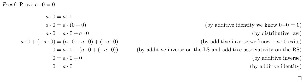
My attempt to prove 1 * 0 = 0, hopefully it is correct ...
The next set of axioms pertain to ordering on the reals which will be helpful in proving some theorems that will follow next:
ORDER AXIOMS on $\mathbb{R}$:
- Given $a,b\in\mathbb{R}$, either $a\leq b$ or $b \leq a$
- If $a\leq b$ & $b\leq a$, then $a=b$
- If $a \leq b$ & $b \leq c$, then $a \leq c$ (i.e. $\leq$ is transitive)
- If $a \leq b$ & $c\in \mathbb{R}$, then $a+c \leq b+c$
- If $a\leq b$ & $0\leq c$, then $ac \leq bc$
All the axioms from before are required to build up the set of properties I am about to present to you, 7 ordering properties that will be essential in your mathematical career. I cannot stress this enough, knowing these properties will help you solve proofs relating to inequalities in this course and in all future courses:
Theorem: properties of an ordered field
- if $a \leq b$, then $-b \leq -a$
- if $a \leq b$ & $c\leq 0$, then $bc \leq ac$
- if $0 \leq a$ & $0 \leq b$, then $0\leq ab$
- $0 \leq a^2$
- $0 \lt 1$
- if $0 < a$, then $0 < a^{-1}$
- if $0 < a < b$ then $0 < b^{-1} < a^{-1}$ for $a,b,c\in\mathbb{R}$
Math is a subject that builds on top of itself so every concept you learn is built on top of other concepts (except for the axioms). How I view Mathematics (Mathematicians, please don’t kill me) is that each theorem and corollary is another tool to solve more difficult problems. But it is also fun to ponder about to see why a particular theorem is true and thus one should try proving one of these properties listed above at least once. I find the first and 7th property particularly useful when working on inequalities. Notice the 7th property explicitly adds a restriction that this property only holds in the reals, there’s a reason for this.
Suppose we have a field with the elements 0,1,2 under modular arithemtric ($F_3$):
| x | 0 | 1 | 2 |
|---|---|---|---|
| 0 | 0 | 0 | 0 |
| 1 | 0 | 1 | 2 |
| 2 | 0 | 2 | 1 |
Multiplication table for $F_3$= {0, 1, 2} under arithmetic mod 3
1 < 2 but in $F_3$, their inverse is itself so if proposition 7 was true then $0 < 1 < 2 \implies 0 < 2^{-1} < 1^{-1} \equiv 0 < 2 < 1$ which is a CONTRADICTION. Funny how I never realised that proposition 7 only holds true for the reals (and perhaps on any ordered field) when I took the course but now reviewing the course content years later made me realise this. Another example of how the little details matter in Mathematics.
The next theorem introduced relates to the absolute value operator, but first we must define what an absolute value is:
Absolute Value: If $a\in\mathbb{R}$ then the absolute value of $a$ is: \(|a| = \begin{cases} a & \text{, if } a\geq 0 \\ -a & \text{, if } a \lt 0 \\ \end{cases}\)
I have seen many students not registering in their brain this definition which ends up biting them later in the course whether it’s a proof question or solving some straightforward math question. Even I am guilty of this myself, forgetting that the following question has two solutions for instance:
\[\begin{align*} x^2 &= 4 \\ \sqrt{x^2} &= \sqrt{4} \\ |x| &= 2 \end{align*}\]This means $x$ can either be -2 or 2. The important thing to take away is that $\sqrt{x^2} = (x^2)^\frac{1}{2} \ne x$ but rather $|x|$. The issue with the exponent laws is that it deletes crucial metadata/information and assumes $x>0$ (i.e. that x is positive).
Theorem: $\forall a, b \in\mathbb{R}$,
- $|a| \ge 0$
- $|ab| = |a||b|$
- $|a+b| \le |a| + |b|$ (Triangle Inequality)
All 3 properties of the theorem are important to know but the triangle inequality stands out the most. It is one of the three distinguishing axioms that defines whether or not a function $d(x,y)$ is a metric, something taught in MATH3001 (or in MATH2000 if you have Jaworski). The most important hint I can give about the proof of the triangle inequality is the following: $-|x| \le x \le |x| \forall x\in\mathbb{R}$.
Bounds
The content covered thus far has been constructing basic properties of mathematical operations involving addition, multiplication, ordering and absolute values. Well the next set of content will be on bounds, a central topic if you are interested in analysis. But first we need to go over some notations and definitions:
Let $S\subseteq \mathbb{R}$ be a nonempty set:
Max: a number $s_o$ is called a MAXIMUM of $S$ if it satsifies the following:
- $s_o\in S$
- $s\le s_o \forall s\in S$
Thus $s_o = \max S$
Min: a number $s_o$ is called a MINIMUM of $S$ if it satisfies the following:
- $s_o \in S$
- $s_o \le s \forall s\in S$
Thus $s_o = \min S$
One important note is that some sets may not have a min or a max such as $(a, \inf) = \{x\in\mathbb{R} | a \lt x \}$ does not have a max nor a min. However, every finite set in $\mathbb{R}$ has a max and a min. To prove that $(a, \inf)$ has no min, it is important to use the definitions above to show otherwise. For instance, I would begin by assuming a min $s_o$ exists and then proceed to specially craft a number such as the midpoint between $a$ and $s_o$ (i.e. $\frac{s_o+a}{2}$ and show that this is first in the set first before showing that it is in fact smaller than our supposed min $s_o$. The same idea can be applied to show a max does not exist in the set. Though I haven’t done any max/min proofs in a while so I could be wrong in the details but the main takeaway is that you need to use the definitions to disprove the existence of a max or min.
UPPER BOUND: If $M\in\mathbb{R}$ satisifies $s\le M \forall s\in S$, then $M$ is called an UPPER BOUND for S and we say $S$ is bounded above
LOWER BOUND: If $M\in\mathbb{R}$ satisifies $m\le s \forall s\in S$, then $M$ is called an LOWER BOUND for S and we say $S$ is bounded below
BOUNDED: If a set $S$ is bounded below and above, we say the set $S$ is BOUNDED
Example: While $(a, \infty)$ does not have minimum, $a$ will be the lower bound since all elements in the set has to be greater than $a$. The set has no upper bound and thus is not a bounded set.
However, the problem with our definitions of upper and lower bound is that there could be many upper and lower bounds for the set. For instance, the finite set with two elements $S = \{0, 1\}$ has infinitely many number of upper and lower bounds in $\mathbb{R}$. I could say 100, or even a 1000 is an upper bound to the set $S$ and -1000 is a lowerbound to S. There’s no utility to this statement. It’s as vague as telling someone “I’m thinking of a number greater than 0” and expecting them to identify it intelligently in one guess. There are infinitely many numbers one could select and serves no purpose aside being vague to ensure the player never had a decent chance to win the game from the start.
(though if you were to play this game, it would be devilish to choose a large interval whereby their chances of getting the answer is so small that there was no point of playing the game to begin with)
This is where our next set of definitions becomes useful in describing upper and lower bounds:
Let $S\subseteq \mathbb{R}$ be nonempty:
- If $S$ is bounded above and has a least upperbound, the least upperbound is called the supremum of $S$ denoted as $\sup S$
- If $S$ is bounded below and has a greatest lowerbound, the greatest lowerbound is called the infimum of $S$ denoted as $\inf S$
More formally,
SUPREMUM: $M = \sup S$ if the following two conditions holds true:
- $\forall x\in S, M\ge x$ (i.e. $M$ is an upperbound of $S$)
- If $N$ is some other upperbound of $S$, then $M\le N$
INFIMUM: $m = \inf S$ if the following two conditions holds true:
- $\forall x\in S, m\le x$ (i.e. $m$ is a lowerbound of $S$)
- If $n$ is some other lowerbound of $S$, then $n \le m$
Though sometimes it is good to replace the 2nd condition of both supremum and infimum with the contrapositive to show that if a potential candidate is smaller/greater than the supremum and infimum, it is actually not a upper/lower bound respectively. For instance, for supremum, we could rewrite the second statement as:
If $N < M$, then $\exists s\in S$ such that $N < s$ (i.e. N is actually not an upperbound)
The reason why this definition is more valuable is that the original statement was indicating that the supremum is the smallest upperbound out of all the upperbounds to the set. This can be extremely difficult or impossible to prove and hence we take the contrapositive. This reduces the problem to just proving that any specific candidate $N < M$ would in fact not be an upperbound which is a much more manageable problem.
Question: Does the supremum need to exist in the set $S$?
Answer: No it does not. Unlike the maximum of a set which must lie in the set itself, there is no restriction in our definition that requires the supremum (nor infimum) to be itself a member of the set.
Example: $S = \{ x\in\mathbb{R} | x < 2\}$ has a supremum $\sup S = 2$ where $2\notin S$
But is this always the case? What property do we need such that any set $S$ has a supremum? And where where would the supremum lie in? For instance, what common number sets/space would be sufficient to encapsulate this.
The naturals and integers obvious bad choices to gaurantee a supremum due to its inability to represent fractions. But the rationals, our set of fractions $\mathbb{Q}$ can infinitely get close to any numbers in $\mathbb{R}$. In fact, between any two rationals, there’s always another rational. Furthermore, there are infinitely numhber of rationals between two rationals (this is refered to as the Density of $\mathbb{Q}$. Surely this would be a good candidate. However, note the wording: $\mathbb{Q}$ can infinitely get close to any numbers, this does not meant it can represent the number itself despite how dense $\mathbb{Q}$.
Like how there is an opposite force for everything, there exists irrational which are equally as dense i.e. between two real numbers, there exists an irrational number. These “gaps” in $\mathbb{Q}$ explain why $\mathbb{Q}$ is not sufficient for our question.
Here’s a simple classical counterexample to this:
$ S = \{ x\in\mathbb{R} | x \le \sqrt{2} \} $
The $\sup S = \sqrt{2}$ but the irrational number $\sqrt{2}\notin \mathbb{Q}$ and thus the set has no supremum over $\mathbb{Q}$ which Mathematicians term to be not complete.
The COMPLETENESS AXIOM: Every non-empty set of real numbers which is bounded above has a least upperbound (supremum) which is an element of $\mathbb{R}$
i.e. If $S\subseteq \mathbb{R}$ is bounded above, $\sup S$ exists and is a real number
The $\mathbb{R}$ does not have such gaps as $\mathbb{Q}\subset\mathbb{R}$ and similarly with the irrationals $\mathbb{I}\subset\mathbb{R}$. In fact $\mathbb{R} = \mathbb{Q} \cup \mathbb{I}$.
As a corollary, the same statement can be made about the infimum:
Corollary of the Completeness Axiom: If $S\subseteq \mathbb{R}$ is bounded below, then $\inf S$ exists and $\inf S\in\mathbb{R}$
As a consequence of the completeness axiom (actually a lot of things derive or require the complete axiom to be true), we can claim no matter how big a number $b$ is, one can choose any positive number $a$ (even an incredibly small one) such that it can be added to itself enough times to dwarf b. This is what Mathematicians call the Archimedean Property:
Archimedean Property: If $a > 0$ and $b > 0$ then $\exists n\in\mathbb{N}$ such that $na > b$
The proof is left as an exercise to the readers (or attend class) but one can use proof by contradiction by supposing that the property itself fails implying $b$ itself is an upperbound of $S = \{ na | n\in \mathbb{N} \}$ and thus by completeness, $M = \sup S$ exists. THen you could reasonably say $M-a < M$ then proceed to show that there must exist some $n\in\mathbb{N}$ such that $na > M-a$ and “magically” show that in fact that M is less than an element in the set S so M cannot be an upperbound of S. That’s the sketch of the proof, you can fill in the blanks yourself.
As a consequences of the archimedean property, we have:
- If $a > 0, \exists n\in\mathbb{N}$ such that $\frac{1}{n} < a$ (i.e. there will always be someone smaller than yourself or in mathematical terms, there is always a fraction smaller than your number)
- If $b > 0, \exists n\in\mathbb{N}$ such that $b < n$ (i.e. equally there will always be someone greater than yourself)
The archimedean property and its consequences are beautiful concepts that we can take to heart. Firstly that no matter how bad you are, there’s always someone will do worse than you and inveresly, no matter how much better you think you are, there’s always someone better than you. Share one of the two consequences to a friend depending on the context. If a classmate or collegue is being obnoxious about how much better they are than you, give them the second consequence. If someone is depressed about their outlook in life, share them the first consequence, though I don’t know how effective that would. Thank goodness I am not a counsellor.
Sequences
A sequence as you already know is an infinite list of numbers but more formally:
Sequences: a sequence is a function from the set of integers larger than some $m\in\mathbb{Z}$ into $\mathbb{R}$:
$S:\{n\in\mathbb{Z} | n \ge m \} \to \mathbb{R}$
$S(n) \to S_n$
Example: Take the sequence that alternates between -1 and 1: $(-1, 1, -1, 1, -1, 1, \ldots )$
We can define an element in the sequence as $a_n = (-1)^n \forall n\in\mathbb{N}$. To represent the sequence: $(a_n)^\infty_{n=1}$.
As this is a course in Calculus, limits are at the heart of everything we do in this course.
Limit of a Sequence: A sequence $(s_n)$ of real numbers converges to a real number $L $ if $ \forall \epsilon > 0, \exists N\in\mathbb{N}$ such that $n > N \implies |s_n-L| < \epsilon$
- if $(s_n)$ converges to L, $\lim_{n\to\infty}s_n = L$ or $s_n \to L$ and we call the number $L$ the limit of $(s_n)$
- if a sequence does not converge then we say the sequence $s(n)$ diverges
- Note: a sequence cannot have more than one limit. It either has a limit or does not.
In a more condensed form:
$\lim\limits_{n\to\infty}s_n = L \iff \forall \epsilon > 0, \exists N$ such that $n > N \implies |s_n - L| < \epsilon$
The formal definition of limits of a sequence is a mouthful but we can informally translate this as:
for any positive number $\epsilon$, no matter how small it is, we can find a number $N$ large enough such that whenever $n > N, s_n$ is a distance less than $\epsilon$ from our limit $L$
Note: $|s_n - L|$ represents the distance between $s_n$ and $L$
It is important that you understand this definition conceptually because this is one of many types of proofs you will see in this course. At the same time, do not panic if you struggle to use this formal definitions to prove a limit because the definition of limits for sequences is quite similar with the limits of a function and what it means for a function to be continuous and even uniformly continuous. While there are nuances between sequences, functions, and uniform continuity, the core idea is the same: for any $\epsilon > 0$, everything eventually stays within an $\epsilon$-window of the limit. Once you master the proofs to one of the 3 or more limit definitions covered in the course, you’ll master all of them.
A visual view of the epsilon window where the sequence converges to L after $n>N$
In these types of proof, the positive number $\epsilon$ must be arbitrary (i.e. not fixed). Thus your task as the prover is to find an $N$ which makes any term of the sequence after $N$ to be within this epsilon window. A fixed $N$ that works for one $\epsilon$ will generally fail for a smaller one — your $N$ must be a function of $\epsilon$.
Here’s a simple rough example to give you an idea: Prove that $\lim\limits_{n\to\infty}\frac{1}{n}=0$
It is often not evident what $N$ to choose, so we start with a rough work and later rewrite our proof more formally. In rough work, we assume the conclusion and work backwards to discover what $N$ should be. Then in the formal proof, we revevrse the direction by defining what $N$ is first and then show the implication holds forward.
Rough Work: Let $\epsilon > 0$ be given. We want to find $N$ such that $n > N\implies |\frac{1}{n}-0|<\epsilon$. Assuming the conclusion hold true, we have:
\[|\frac{1}{n} - 0| = |\frac{1}{n}| = \frac{1}{n} < \epsilon \nonumber\]For the above statement to occur:
\[\frac{1}{n} < \epsilon \iff 1 < n\epsilon \iff \frac{1}{\epsilon} < n \nonumber\]Thus we will choose $N=\frac{1}{\epsilon}$. I will leave the formal proof as an exercise to you the readers, most of the work has already been done.
As previously, mentioned, a sequence cannot have more than one limit. It either has a limit or does not.
Theorem: Let $s(n)$ be a sequence of real numbers. Then $\lim\limits_{n\to\infty}s_n=$ and $\lim\limits_{n\to\infty}s_n=t \implies s = t$
Originally, I wanted to leave the proof as an exercise but the proof involves a technique extremely important in Mathematics that I could not pass it.
Proof: Suppose $\lim\limits_{n\to\infty}s_n = s$ and $\lim\limits_{n\to\infty}s_n=t$ Let $\epsilon > 0$ then $\frac{\epsilon}{2}$ is also greater than 0 as well. We apply the definition of convergence to $\frac{\epsilon}{2}$.
We can have our $\epsilon$ window to be $\frac{\epsilon}{2}$ because $\epsilon$ is arbitrary and therefore it can be as arbitrarily small as we want it to be. In simpler terms, we just renamed $\epsilon$ as $\frac{\epsilon}{2}$
Then $\exists N_1$ such that $|s_n-s|<\frac{\epsilon}{2}, \forall n > N_1$ (*)
Then $\exists N_2$ such that $|s_n-t|<\frac{\epsilon}{2}, \forall n > N_2$ (**)
Let $N=\max{N_1, N_2}$, this is a technique often employed when there are multiple numbers to consider in these limit types proof.
If we want to prove that s = t, that is equivalent as saying its difference, or rather distance is 0: $|s - t| = 0$
However, we have no direct way to relate s and t to each other. The only information we have thus far is that they are both limits to the same sequence $(s_n)$. So the question is how can we relate s and t in a way that involves the sequence. This bridge it turns out is our magical number 0. This is a powerful technique whereby adding or subtract 0 has zero impact in the equation yet has profound effect to our consciousness.
\[\begin{align*} |s - t| &= |(s + 0 - t)| \\ &= |s + (-s_n + s_n) - t| \\ &= |(s - s_n) + (s_n - t)| \\ \end{align*}\]The effect of introducing an intermediate term that cancels out transforms a once stagnant problem into something that gives hope to us that we are one step closer to our objective. What is great about rigorous introductory courses is how well-structured the course is, building up concepts from the ground up. We have started with fields, ordering and eventually to the triangle inequality. Currently, we can see some semblance of our limits from (*) and (**) but not quite exactly in the form we desire. This is where a student should stop and reflect what has been covered in the course thus far and try to pull out tools and tricks to manipulate the problem to our advantage and the triangle inequality is one of such tools.
Recall the triangle inequality tells us that $|a + b| \le |a| + |b|$, so if we take $a = s-s_n$ and $b = s_n - t$, then we can invoke the triangle inequality as follows (I like to imagine if magic was real, it would be very scientific and mathematical in nature):
\[\begin{align*} |s - t| = |(s - s_n) + (s_n - t)| \le |s - s_n| + |s_n - t|\\ \end{align*}\]If we are trying to prove that the limit $s, t$ of the same sequence are equal to each other, we must have this inequality be less than some $\epsilon$-window. What may not be obvious at first glance is that $|s - s_n|$ and $|s_n - s|$ are the same thing. Taking the absolute difference of two numbers measures distance and distance are symmetric (one of the three properties of a metric) but for those who have a hard time seeing this:
\[\begin{align*} |s - s_n| &= |(-1)(-s + s_n)| \\ &= |(-1)(s_n - s)| \\ &= |-1||s_n - s| \\ &= (1)|s_n - s| \\ &= |s_n - s| \end{align*}\]Therefore, we now have the following:
\[\begin{align*} |s - t| \le |s_n - s| + |s_n - t| \end{align*}\]If $n>N$, both (*) and (**) are true, then for $n > N$, we now have:
\[\begin{align*} |s - t| \le |s_n - s| + |s_n - t| < \frac{\epsilon}{2} + \frac{\epsilon}{2} = \epsilon \end{align*}\]Since $|s - t| < \epsilon$ for all positive number $\epsilon$, we must have $|s - t| = 0 \implies s = t$ as needed.
If a sequence does not have a limit, how do we show the sequence does not converge? It turns out we must find at least one value of $\epsilon$ for which the definition fails.
Example: Show that the sequence $(s_n)$ does not converge where $s_n = (-1)^n$.
This an alternating sequence between -1 and 1. Let’s pick $\epsilon=1$ and if that doesn’t work we’ll revise it later. Notice that the distance between $|1 - (-1)| = 2$ thus we need to choose an epsilon window $2\epsilon \le 2$ to guarantee that 1 and -1 cannot both fit inside this window simultaneously. That is the intuition behind choosing $\epsilon=1$.
The goal is to for the $\epsilon$ I pick, I cannot find an $N$ such that $|s_n - L| < \epsilon=1 \forall n > N$.
Suppose by contradiction that $\lim\limits_{n\to\infty}s_n = L, L\in\mathbb{R}$. Since $\epsilon = 1 > 0, \exists N$ such that $n > N \implies |s_n - L| < 1$. Thus we have:
\[|(-1)^n - L| < 1 \nonumber\]We can break the sequence into two cases:
- n is even: $|1 - L| < 1$
- n is odd: $|-1 - L| = |-1(1+L)| = |1 + L| < 1$
We know that the distance of two neighboring terms in the sequence has a distance of 2 and thus:
\[2 = |1 + 1| = |1 (-L + L) + 1| = |(1-L) + (1+L)| \nonumber\]Notice a pattern? Earlier we showed how introducing an intermediate term that cancels each other out had a profound impact to manipulate our equation to something closer to our desired outcome. Then we had invoke the triangle inequality, the same can be repeated again in this question:
\[|(1-L) + (1+L)| \le |1-L| + |1 + L|\nonumber\]Now we have the two even-odd cases of our sequence that can be substituted into the equation: \(|(1-L) + (1+L)| \le |1-L| + |1 + L| < 1 + 1 = 2 \nonumber\)
Thus far we have shown $2 \le |1 - L| + |1 + L| < 2$ which is a contradiction. Therefore, no such $L\in\mathbb{R}$ exists and $(-1)^n$ does not converge (i.e. it diverges)
Similarly how we showed a set can be bounded, we can equivalently show a sequence can be bounded as well.
Note The difference between a set and a sequence are the following:
- sets containly only unique elements meanwhile a sequence can repeat the same number many times
- sets are not ordered but the position of each element in the sequence matters
- sets are finite meanwhile sequences have infinitely many elements
Bounded Sequence: A sequence $(s_n)_{n=m}^\infty$ is called BOUNDED if the set $\{s_n | n \ge m \}$ is bounded
Equivalently, $(s_n)^\infty_{n=m}$ is bounded $\iff \exists M > 0$ such that $|s_n| \le M \forall n$
Here are some noteworthy theorems of sequences that I think are interesting to remember, albeit perhaps a bit informally. You have seen these be called the limit laws elsewhere. The proofs are left as an exercise (or attend the class or read the textbook).
Theorem: $\lim\limits_{n\to\infty} k s_n = k \lim\limits_{n\to\infty} s_n$ for some $k\in\mathbb{R}$
Theorem: $\lim\limits_{n\to\infty} (s_n + t_n) = \lim\limits_{n\to\infty}s_n + \lim\limits_{n\to\infty}t_n$ provided both converges
Theorem: $\lim\limits_{n\to\infty}s_nt_n = (\lim\limits_{n\to\infty}s_n)(\lim\limits_{n\to\infty}t_n)$ provided both converges
Theorem: $\lim\limits_{n\to\infty}\frac{s_n}{t_n} = \frac{\lim\limits_{n\to\infty}s_n}{\lim\limits_{n\to\infty}t_n}$ as long as $\lim\limits_{n\to\infty}t_n \ne 0$
Theorem: $\lim\limits_{n\to\infty}s_n^{-1} = \frac{1}{\lim\limits_{n\to\infty}s_n}$ as long as $\lim\limits_{n\to\infty}s_n \ne 0$ and converges
What the limit laws permit us is to determine the limit of a sequence very quickly. The $\epsilon-N$ method is essential for proving results from first principles and is often much difficult method whereas the limit laws let us compute limits quickly provided convergence is established (but its often assumed in non-rigourous courses). Here are some limits whose proofs will be left as an exercise:
- $\lim\limits_{n\to\infty}\frac{1}{n^p} = 0$ for $p > 0$
- $\lim\limits_{n\to\infty}a^n = 0$ if $|a| < 1$
- $\lim\limits_{n\to\infty}n^\frac{1}{n}=1$
- $\lim\limits_{n\to\infty}a^\frac{1}{n} = 1 \quad \forall a > 0$
To prove one of the limits listed above, an important concept called the squeeze theorem needs to be introduced.
Squeeze Theorem: if $s_n \le t_n \le r_n$ and $s_n \to L, r_n \to L$ then $t_n \to L$
The squeeze theorem (also called the sandwich rule) is literally what it sounds like, if a sequence is bounded below and above by two different sequences and the two different sequences converge to the same number then by effect, the sequence we are working on also converges to the same number.
A common theme you will find in calculus and in analysis in general is that things can have infinite limits i.e. is unbounded. For instance, the sequence $(n^2)$ is unbounded and thus does not converge (i.e. diverges to infinity). An infinite limit is another way of saying it diverges to infinity or negative infinity.
Infinite Limits: For a sequence $(s_n)$, we say $\lim\limits_{n\to\infty}s_n = \infty$ if for every $M > 0, \exists N $ such that $n > N\implies s_n > M$ (i.e. diverges to \infty$
In plain language, no matter what $M$ you pick, you can always find a bigger number in the sequence
Of course there is the negative infinity version of this definition and yes I know it sounds ridiculous at first to prove something does not converge. Previously, we have stated that to prove something does not diverge, it suffices to find one single $\epsilon$ such that the epsilon window cannot be true. It turns out that there are sequences, series and functions whose convergence is still a mystery such as the flint hill series:
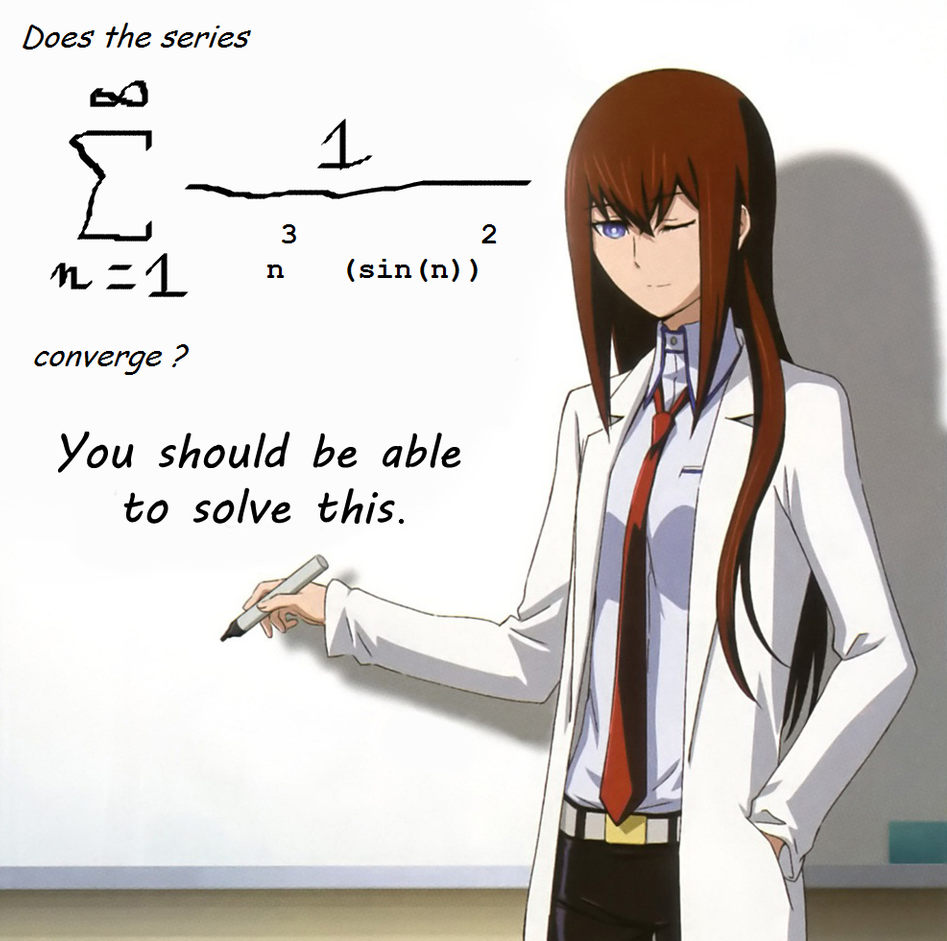
Kurisu from Steins;Gate challenging the audience to solve a series whose convergence is not yet known by the Mathematical community. Source: reddit
Non-convergence does not imply a sequence has no limits. It simply means that the sequence does not converge to a single real number.
Existence of a Limit: A sequence $(s_n)$ has a limit (i.e. a limit exists) if either:
- $s_n$ converges
- $s_n$ diverges to $+\infty$
- $s_n$ diverges to $-\infty$
Let’s now look at an example of proving $(n^2)$ has a limit even if it cannot be bounded:
Example: Show $\lim\limits_{n\to \infty}n^2 = \infty$
Sketch/Rough Work: Given $M > 0$, we need to find $N$ such that for $n > N$, we have:
\[\begin{align*} n^2 &> M \\ \sqrt{n^2} &> \sqrt{M}, \qquad M > 0\\ n &> \boxed{\sqrt{M} = N}, \quad n > 0 \end{align*}\]Proof: Let $M > 0$ and choose $N=\sqrt{M}$.
Then for $n > N \implies n > N = \sqrt{M}$ and as $n, M > 0$:
$n^2 > M$ as required.
Now that we established the existence of infinite limits, we now have the following limit law as a consequence:
Theorem: Let $(s_n)$ be a sequence of positive numbers. Then $\lim\limits_{n\to\infty}s_n = \infty \iff \lim\limits_{n\to\infty}\frac{1}{s_n} = 0$
Before we proceed to the next topic, it is important to note that $\pm\infty$ are not real numbers and thus the limit laws that we became familiar with do not apply. In fact, we will soon learn that we call these indeterminate forms (e.g. $\infty - \infty, \frac{\infty}{\infty}, and 0\cdot\infty$). If you are fortunate enough, you will learn that not all infinities are treated equal. There are different classes of infinities and some are larger than the others.
Let us now proceed to finding tools or other methods to show a given sequences converges without knowing the limit in advance. Often times even with the formal definition, we discover the limits upon trying to prove the statement. But surely, there is a better way and yes there is but it only occurs for a certain subclass of sequences.
Before we learn this magical spell, we first need to define what it means for a sequence to be increasing and decreasing.
A sequence $(s_n)$ is said to be:
- INCREASING: if $s_n \le s_{n+1} \forall n$
- DECREASING: if $s_n \geq s_{n+1} \forall n$
Notice that the definitions does not imply the sequence is strictly increase nor strictly decreasing via the usage of $\le$ and $ge$ in lieu of $\lt$ and $gt$ in their definition. This implies a straight constant line is both always increasing and always decreasing. Weird right?
If a sequence is always increasing or always decreasing, it is called monotonic (i.e. can only go in one direction). Restricting a sequence to be monotonic AND bounded leads us to the following theorem:
Theorem: Any bounded monotone sequence converges
Let’s consider why the theorem requires boundness and that the sequence is monotonic:
- without boundness, the sequence can diverge to $\pm\infty$ and thus does not converge
- without montonic property, we could have a bounded sequence that jumps/alternates between two numbers and thus never truly converges to a single real number (i.e. $((-1)^n)$ alternates between -1 and 1
Here’s a question that I myself got wrong when reviewing the material:
Question: Suppose we have a sequence where the distance between each subsequent neighbor gets closer and closer to each other. Does this sequence converge? Answer: No it does not, the two terms could be inching towards each other so slowly that convergence is not guaranteed
Thus, this brings us to the next type of sequences: cauchy sequences
Cauchy Sequences: a sequence $(s_n)$ is called a CAUCHY sequence if $\forall \epsilon > 0, \exists N$ such that for all $m,n > N \implies |s_n - s_m| < \epsilon$
What Cauchy sequence is telling us is that as $m, n$ get large, $s_n, s_m$ get closer and closer to each other. An important note is that $s_n$ and $s_m$ do not have to be neighbors. It’s as if there’s a clustering whereby the terms are getting closer and closer to each other, where a bunch of terms are being compressed more and more to each other.
This increasing clutering of points allows us to make the following statement:
Theorem: A sequence is convergent $\iff$ it is a cauchy sequence
We now have two tools (theorems) we can use to determine whether or not a sequence converges or not without finding its limit. This implies we can use our beloved limit laws without explicitly proving convergence.
Previously, we stated that every bounded monotone sequence converges. We also discovered that without monotonic property, convergence is no longer a guarantee. But what if we look at its subsequence?
For $s_n = (-1)^n$, the sequence $(s_n)$ does not converge as it alternates between -1 and 1. But if we were to filter every 1st or 2nd term, we obtain a new subsequence of a list of -1 or 1 respectively and those converge. But before we explore the implication of convergence i.e. does every subsequence converge? we first need to define what a subsequence is:
Subsequence: let $(s_n)$ be a sequence. Then a sequence $(t_k)_{k\in\mathbb{N}}$ is called a subsequence of $(s_n)$ if for each $k\in\mathbb{N}, \exists n_k$ such that $n_1\lt n_2\lt n_3\lt\cdots$ and $t_k=s_{n_k}$
Since we can chose any terms in order when creating a subsequence, it should come as to no surprise of the following:
Theorem: Every sequence has a monotone subsequence
Since any sequence has a monotone subsequence, what can we say about convergence? It turns out that:
Bolzano-Weierstrass Theorem: every bounded sequence has a convergent subsequence
Recall how the monotonic convergence theorem required the sequence to be both monotonic and bounded? Since every sequence has a montonic subsequence and if we create a monotonic subsequence from a bounded sequence, then it surely comes no surprise that the subsequence is also bounded. Since the subsequence is monotone and bounded, the monotone convergence theorem guarantees it converges.
Bolzano-Weierstrass theorem implies the following:
Theorem: Cauchy sequences are bounded
Though I think that was already obvious, if all cauchy sequences are convergent to a single value, there’s no way it is not bounded either. Of course, I will like to stress, being bounded does not imply convergence at all.
What may not be obvious is whether the subsequence of a convergent sequence converges to the same limit (at least it is not obvious till you are reminded what it means to converge to a limit $L$). The answer is yes (actually in hindsight this should have been obvious but my little brain didn’t think it was):
Theorem: If $(s_n)$ converges to $L$ then every subsequence converges to $L$ as well
As I alluded to previously, we will be also studying the convergence of series, specifically of infinite series but first we need to define what partial sums are:
Partial Sums: $s_n = \sum\limits_{k=m}^n a_k = a_m + a_{m+1} + \ldots + a_n$
Partial sums is simply a finite sum of numbers in a series.
An infinite series is said to converge if the sequence of partial sums $(s_n)$ converges to a real number: $\sum^\infty_{n=m} a_n = s \iff \lim_{n\to\infty}s_n = s \iff \lim\limits_{n\to\infty}(\sum\limits_{k=m}^n a_k) = s$
In simpler terms, if the sequences of partial sum converges then the infinite sum converges as well.
Some Common Series:
- Geometric Series: $\sum\limits_{n=0}^\infty r^n = \frac{1}{1-r}$ where $|r| \lt 1$
- Harmonic Series: $\sum\frac{1}{n}$ diverges
- P-Series: $\sum\frac{1}{n^p}$ converges if $p > 1$ and diverges if $p \le 1$
The harmonic series is an interesting case because intuitively, one would imagine it converges. Recall that any bounded monotone sequence converges. When we look at the sequence $s_n = \frac{1}{n}$ is indeed bounded between 0 and 1 and is monotonically decreasing. In fact it is intuitively obvious that $\lim\limits_{n\to\infty}\frac{1}{n} = 0$. While the sequence converges, the (harmonic) series does not. We will later show why the harmonic series diverge soon with the comparison test though there are many ways to show that the series diverge (e.g. the integral test taught in MATH2052).
Unlike with sequences where one could skip the first $N-1$ terms, series requires us to aggregate every single term in the series. Thus while one may be tempted to adopt intuition from sequences to series. This does not work. Perhaps it is just me, but my initial intuition was nudging me that since the terms were approaching to 0 at a relatively decent pace, the series could be bounded above. However, if one was to write the first few terms, they’ll quickly realise this cannot be the case as we can always find a grouping of terms that sum greater than 1/2:
\[\begin{align*} \sum_{n=1}^{\infty} \frac{1}{n} = 1 + \frac{1}{2} + \underbrace{\frac{1}{3} + \frac{1}{4}}_{> \frac{1}{2}} + \underbrace{\frac{1}{5} + \frac{1}{6} + \frac{1}{7} + \frac{1}{8}}_{> \frac{1}{2}} + \underbrace{\frac{1}{9} + \cdots + \frac{1}{16}}_{> \frac{1}{2}} + \cdots \end{align*}\]The main issue is that $\frac{1}{n}$ grows much faster than desired for convergence and hence why the p-series requires that the power $p$ is greater than 1.
Comparison Test: Let $\sum a_n$ be a series with $a_n\ge0\forall n$
- if $\sum a_n$ converges and $|b_n| \le a_n \forall n$, then $\sum b_n$ converges (i.e. if the car ahead of you stops, you as well will stop)
- If $\sum a_n = \infty$ and $b_n \geq a_n \forall n$, then $\sum b_n = \infty$ (i.e. suppose you are in a one way road and the car behind you is always tailing you without slowing down, you also cannot slow down either)
I no longer recall who told me the car analogy, but it’s one simple way to remember the comparison test.
The issue with comparison test is that it requires us to already know good candidates to consider that converges or diverges already. Though we already know 3 types of series that can either converge or diverge making our lives much easier. Here’s a simple example in action:
Example: $\sum\limits_{n=1}^\infty \frac{1}{n^2+1}$. Does it converge or diverge
By p-series we know that $\sum \frac{1}{n^2}$ converges since $p > 1$. Thus we have:
\[\begin{align*} \sum\limits_{n=1}^\infty \frac{1}{n^2+1} \lt \sum\limits_{n=1}^\infty \frac{1}{n^2} \forall n \end{align*}\]Thus by comparison test $\frac{1}{n^2 + 1}$ also converges.
Absolute Convergence: a series $\sum a_n$ converges absolutely if $\sum |a_n|$ converges
- if $\sum |a_n|$ diveres but $\sum a_n$ converges, we say $\sum a_n$ converges conditionally
By implication, it is obvious that absolute convergence implies convergent but it does NOT apply in the reverse direction.
convergent $\nRightarrow$ (DOES NOT imply) absolute convergence
Proof: $\sum\frac{(-1)^n}{n}$ converges conditionally but $\sum |\frac{(-1)^n}{n}| = \sum\frac{1}{n}$ (a harmonic series) does not diverge by p-test
Ratio Test: let $\sum a_n$ be a series of non-zero terms for which $\lim\limits_{n\to\infty}|\frac{a_{n+1}}{a_n}| = L$ exists. Then:
- $\sum a_n$ converges absolutely if $L < 1$
- $\sum a_n$ diverges if $L \gt 1$
- $\sum a_n$ may either converge or diverge if $L = 1$
As the name implies, the ratio test compares what I view as the eventual growth behaviours of consecutive terms in the series. If the growth is less than 1, it indicates a shrinking behavior where the next term in the series does not dominate the current term. However, when the ratio is greater than 1, then the subsequent term dominates its previous term and hence will not converge i.e. it exhibits a growth pattern. Both growth patterns behave similarly with the geometric series. Take caution that when the limit $L = 1$, it tells us nothing about the series.
Root Test: let $a_n$ be a series for which $L = \lim_{n\to\infty}|a_n|^\frac{1}{n}$ exists. Then:
- if $L \lt 1$, $\sum a_n$ converges absolutely
- if $L > 1$, $\sum a_n$ diverges
- The test fails if $L=1$
One of the beauty of the root and ratio tests is that their conditions behave the same, eliminating the need to remember an extra set of cases.
Alternating Series Test: if $(a_n)$ is a DECREASING sequence of non-negative numbers and $\lim\limits_{n\to\infty} a_n = 0$ then the alternating series $\sum(-1)^{n+1}a_n$ converges
The alternating series test is a bit of a unique case whereby there are two conditions to satisfy before the test can be applied.
Here’s a list of tests in order that one should try when solving the problem of convergence of series:
General Rule of Series Test:
Growth Hierarchy: $n^n \gt n! \gt a^n \gt$ polynomials
$n^n$ root $n!$ ratio $2^n$ root $\frac{p(n)}{q(n)}$ comparison $r^n$ geometric $\frac{1}{n^p}$ p-series $\frac{a^n}{b^n}$ geometric
What does it mean for a function to be continuous? One simple answer is to say that one should be able to draw the curve without ever lifting the pencil. A more sophisticated answer is to say a function is continuous when the function does not contain any holes, jumps or vertical asymptotes. That is to say,
Continuity: A function $f(x)$ is said to be continuous at $x=a$ if the follow conditions are all true:
- $f(a)$ is defined
- $\lim_\limits{x\to a} f(x)$ exists (i.e. $\lim\limits_{x\to a^-} f(x) = \lim\limits_{x\to a^+} f(x)$)
- $\lim\limits_{x\to a} f(x) = f(a)$
However, the definition of limits above is not rigorous enough for us Mathematicians (or wanna-be). Recall that the definition of convergence of a sequence using limits involved an epsilon window and the work involved to determine an index N at which point we guaranteed all subsequent terms are within the $\epsilon$-window? We will be introducing a similar rigorous definition to define what it means for a function $f$ to approach $f(a)$. For functions, instead of $n\to\infty$, we have $x\to a$ and instead of asking whether the distance between the limit $L$ and $s_n$ fits within our $\epsilon$-window, we now ask whether the distance between $f(x)$ and $f(a)$ is infinitely close such that it fits within the $\epsilon$-window. Unlike the sequence which is one dimensional, functions are multi-dimensionals (2-D in our case) requiring an extra variable $\delta$ to specify how close $x$ has to be with $a$ for the distance between function at $a$ and $x$ fit within the $\epsilon$-window.
$\epsilon-\delta$: let $f$ be a real-valued function with domain of f $\subseteq \mathbb{R}$ be the limit of some sequence in domain of f and let $L\in\mathbb{R}$
Then $\lim\limits_{x\to \color{tomato}{a}} f(x) = \color{cornflowerblue}{L}$ means $\forall \epsilon > 0, \exists \delta > 0$ such that $0 < | x - \color{tomato}{a} | < \delta$ and $x\in dom(f) \implies |f(x) - \color{cornflowerblue}{L}| < \epsilon$
The blue band represents the $\epsilon$-window around $f(a)$ on the y-axis. The red band represents the $\delta$-window around $a$ on the $x$-axis. Any $x$ within the $\delta$-window maps to $f(x)$ within the $\epsilon$-window.
Example: Let $f(x) = \frac{x^2-1}{x-1}$. Prove $\lim\limits_{x\to\color{tomato}{1}}f(x) = \color{cornflowerblue}{2}$. Note that $dom(f) = {x\in\mathbb{R} : x \ne 1}$
First observe that this function can be simplified:
\[\require{cancel} \begin{align*} \frac{x^2-1}{x-1} &= \frac{\bcancel{(x-1)}(x+1)}{\bcancel{x-1}}, \quad x \ne 1 \\ &= x+1, \quad x\ne 1 \end{align*}\]Rough Work: Given $\epsilon \gt 0$, we want to find $\delta > 0$ such that
\[\begin{align*} |x - \color{tomato}{1}| \lt \delta &\implies |f(x) - \color{cornflowerblue}{2}| \lt \epsilon \\ \end{align*}\]If $x \ne 1$, then $f(x) = x + 1$:
\[\begin{align*} |f(x) - \color{cornflowerblue}{2}| = |(x+1) - 2 | = |x - 1| \end{align*}\]Recall that we are trying to find the $f(x)$ as $x\to \color{tomato}{1}$ so we can say the following:
\[|f(x) - \color{cornflowerblue}{2}| = |x - 1| < \delta \stackrel{\text{want}}{\leq} \epsilon \nonumber\]So take $\delta = \epsilon$
Proof: Let $\epsilon \gt 0$. Choose $\delta = \epsilon$. Let $x \ne 1 \implies f(x) = x + 1$.
Then for $0 \lt | x - 1 | \lt \delta \implies |f(x) - 2| = |x + 1 - 2 | = |z - 1| \lt \delta = \epsilon$ as required
We’ve thus far discussed sequences in respect to series, so let’s also relate sequences to functions, more specifically, to continuity:
Theorem: let $f$ be a real-valued function with $dom(f)\subseteq\mathbb{R}$ and let $a\in dom(f)$. Then
$f$ is continuous at $a \iff $(for every sequence $(x_n)$ in dom($f$) converging to $a$, we have $\lim\limits_{n\to\infty} f(x_n) = f(a)$)
Though the way I would short-hand this theorem is the following:
Theorem: f is continuous at $a \iff$ for $(x_n) \to a$, we have $\lim\limits_{n\to\infty} f(x_n) = f(\lim\limits_{n\to\infty} x_n) = f(a)$
Let’s work on a problem to illustrate the power of this new theorem by comparing between the classical $\delta-\epsilon$ proof and the theorem:
Example: Prove that $f(x) = 3x^3 - 2x^2 + x + 1$ is continuous on $\mathbb{R}$.
Approach 1: use $\delta-\epsilon$ definition:
- Rough Work: Given $\epsilon > 0$, we must find $\delta > 0$ such that $0 \lt |x - a | \lt \delta \implies | f(x) - f(a) | \lt \epsilon$:
That’s a lot of work and we still have not found a suitable $\delta$ …
Suppose $\delta \lt 1$ such that $|x - a|\lt \delta \implies |x - a| \leq 1$
Using the trick we learnt at the beginning (i.e. the power of adding 0 by inserting terms that cancel each other):
$|x| = |x - a + a | \leq | x - a | + |a| \lt 1 + |a|$
This weird bounding of $|x| \lt 1 + |a|$ may seem weird but this is simply to bound $x$ in terms of a fixed value (constant) $a$ to simplify the long expression we retrieved above:
\[\begin{align*} |f(x) - f(a)| &\leq (|x - a|)(3(1 + 2|a| + |a|^2) + 3|a|^2 + 3|a| + 3|a|^2 + 2 + 2|a| + 2|a| + 1)\\ &\leq \delta(3 + 6|a| + 3|a|^2 + 3|a|^2 + 3|a| + 3|a|^2 + 2 + 2|a| + 2|a| + 1) \\ &\leq \delta(9|a|^2 + 13|a| + 6) \stackrel{\text{want}}{\leq} \epsilon \end{align*}\]Therefore choose $\delta = \min\{\frac{\epsilon}{9|a|^2 + 13|a| + 6}, 1\}$
That was a lot of work just to finish the rough work and find the $\delta$. Let’s now look at using the theorem we learned recently:
Approach 2: Using the theorem (theorem 17.2 in Ross Analysis)
Suppose $a\in\mathbb{R}$ and suppose $\lim\limits_{n\to\infty} x_n = a$. We need to show $\lim\limits_{n\to\infty}f(x_n) = f(a)$:
\[\begin{align*} \lim\limits_{n\to\infty}f(x_n) &= \lim\limits_{n\to\infty}(3x_n^3 - 2x_n^2 + x_n + 1) \\ &= 3\lim\limits_{n\to\infty}x_n^3 - 2\lim\limits_{n\to\infty}x_n^2 + \lim\limits_{n\to\infty}x_n + \lim\limits_{n\to\infty}1 \\ &= 3(\lim\limits_{n\to\infty}x_n)^3 - 2(\lim\limits_{n\to\infty}x_n)^2 + \lim\limits_{n\to\infty}x_n + 1 \\ &= 3 a^2 -2a^2 + a + 1 \\ &= f(a) \end{align*}\]As $f$ is continuous at $a$ and since $a\in\mathbb{R}$ was arbitrary, by the thoerem (17.2), $f$ is continuous on all of $\mathbb{R}$
It is obvious which method was preferrable … (unless you are a machochistic)
As one knows, the function $\cos(x^2+2x)$ is a composite function composed of one or more functions. Most functions we encounter are composed this way, so it is important to understand how composition affects the domain, since continuity at a point is only defined for points within the domain of the function.
Composite Functions: Let $f,g$ be real-valued functions. If $x\in dom(f)$ and $f(x)\in dom(g)$, we define $g \circ f(x) = g(f(x))$.
Then $g \circ f$ is a function defined on $\{x\in dom(f): f(x)\in dom(g)\}$ ($g$ is composed with $f$)
Example:
Let $f(x) = x+ 1$ and $g(x) = x^2$ then:
$(f\circ g)(x) = g(f(x)) = g(x+1) = (x+1)^2$
$g\circ f)(x) = f(g(x)) = f(x^2) = x^2 + 1$
As we can see $f \circ g \ne g \circ f$ in general
Now that we are familiar with composed function and their domain, let us now discuss continuity for composed functions:
Continuity for Composed Functions: If $f$ is continuous at $a$ and $g$ is continuous at $f(a)$ then $g \circ f$ is continuous at $a$
Here are some facts about continuous functions:
- Polynomials are continuous on $\mathbb{R}$
- Rational function ($\frac{p(x)}{q(x)}$ where $p,q$ are poilynomials) are continuous on $\{x\in\mathbb{R} | q(x) \ne 0\}$
- $f(x) = \sqrt{x}$ are continuous
- $\sin x, \cos x, \tan x$ are continuous within their domain
- $e^x, 2^x, a^x \forall a \gt 0$ are continuous on $\mathbb{R}$
- $\log (x), \log_a(x) (a \gt 1), \ln (x) = log_e(x)$ are continuous on $(0,\infty)$
- $f(x) = x^p, \forall p\in\mathbb{R}$ is continuous on $\mathbb{R}$
Suppose we restrict the domain of some function to some closed interval $I$, then we can make the claim that the function is bounded on this interval.
Furthermore, we can also make the claim that the max and min values of the bounded continuous function can be obtained.
Unsurprisingly, since the interval is closed, it is obvious that we can obtain the max and min.
Bounded Functions: let $f$ be a real-valued continuous function defined on the CLOSED interval $[a, b]$. Then $f$ is BOUNDED on $[a, b]$. Furthermore, $f$ assumes its max and min values on $[a, b]$.
This result is absolutely not surprising at all. If we remove the criteria that the function is closed then:
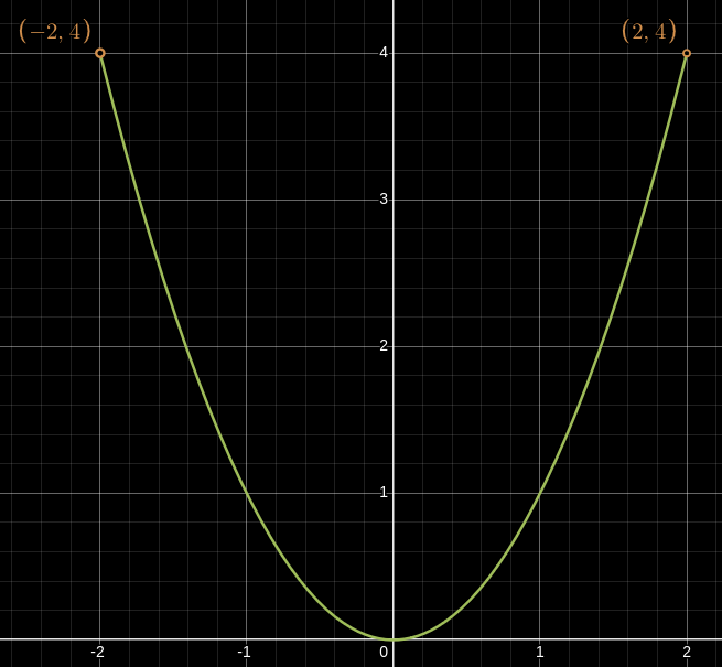
A graph $x^2$ where $x\in(-2,2)$.
In the above graph $x^2$ restricted in the open interval $(-2, 2)$ does not obtains its max since $x = 2 \notin (-2, 2)$.
Thus one can convince themself that for a continuous and bounded function $f$ to obtain its max and min values, it must be restricted on a closed interval. Note that if there was no bounds, the curve $x^2$ only has a minimum at $x = 0$.
Below is an example of the consequence of a curve $x^2$ with a jump at $x = 0$ not obtaining its min despite being closed between $[-2, 2]$ since the curve is not continuous:
![a graph of x^2 where x is restricted to [-2,2] with a jump at x = 0](/assets/math-physics/graphs/x^2-not-continuous.png)
A graph $x^2$ where $x\in[-2,2]$ with a jump at $x = 0$
Though if you are a die-hard theoretical Mathematician, feel free to attempt the proof yourself if you are not sufficiently satisfied with the conclusion.
The next theorem builds on top of the previous theorem on continuous bounded functions. Suppose we are mapping the temperature throughout the day. If in the morning it was $10^\circ C$ and $20^\circ C$ in the afternoon then we can say for certainty that there was some point between the morning and the afternoon where it reached $17^\circ C$. Temperatures don’t magically jump, it increases progressively (I dropped out of physics so I could be wrong).
For American readers, please switch to Celsius
Intermediate Value Theorem (IVT): let $f$ be a continuous and real-valued function on a closed interval $[a, b]$. Suppose that $y$ lies between $f(a)$ and $f(b)$. Then there exists at least one $x\in(a, b)$ such that $f(x) = y$.
A temperature curve showing how between the morning and the afternoon, we can guarantee that there is some time between the two where the temperature is at $17^\circ C$
Uniform Continuity
Previously, our definition of continuity of a function was local in scope, in other words, we could argue that a function was continuous at a particular point. In doing so, we discovered that our $\delta$ depended on both $\epsilon$ window we were trying to satisfy and the specific point we were arguing continuity at. A different point might require a completely different $\delta$ for the same $\epsilon$ window. Hence why when we were trying to show $f(x) = 3x^3 - 2x^2 + x + 1$ was continuous on $\mathbb{R}$, we choose our $\delta$ to be $\min{\frac{\epsilon}{9|a|^2 + 13|a| + 6}, 1}$ where it depended on both the $\epsilon$ and the point $a$. Thus we had infinitely many number of $\delta$ values to apply to show the polynomial function was continuous on $\mathbb{R}$. This is what uniform continuity tries to solve by having $\delta$ only depend on $\epsilon$ and hence have a global scope. Though not all functions are uniformly continuous so it is important some properties of uniform continuity. But first, let’s go through the formal definition of uniform continuity:
Uniformly Continuity on S: let $f$ be a real-valued function on a set $S$. We say $f$ is UNIFORM CONTINUOUS on $S$ if $\forall \epsilon > 0, \exists \delta > 0$ such that $(x, y\in S$ and $|x - y| \lt \delta)\implies |f(x) - f(y)| \lt \epsilon$
i.e. $\delta$ depends only on $\epsilon$ and $x, y$ are abitrary points that are extremely close to each other in the set
Since uniform continuity is not dependent on any single point in the graph but rather requires a single $\delta$ to work for all pairs of points $x, y$ close to each other simultaneously, it is a global property. Any two points that are close in the domain are guaranteed to map to points that are close in the range, regardless of where they sit on the curve.
It should come to no surprise that if $f$ is uniformly continuous on a set $S$ then $f$ is continuous on $S$ since being uniformly continuous is a much stricter definition than continuity. However, the inverse is not true.
$f$ is uniformly continuous on a set $S \implies$ $f$ is continuous on $S$
i.e. uniform continuous $\implies $ continuous
Note: continuity $\bcancel{\implies}$ uniform continuity
We previously saw that if a function $f$ is continuous on a closed interval, it is bounded and attains it max and min. Furthermore, we also discovered the ability to infer the existence of an event occuring if it lies between two different other events via the intermediate value theorem. What could we say about uniform continuity?
Theorem (Bounded Continuous Functions implication on Uniform Continuity): If $f$ is continuous on a closed interval $[a, b]$, then $f$ is uniformly continuous on $[a, b]$
Thus we can say the following:
$f$ is continuous on a closed interval $[a, b] \iff f$ is uniform continuous on $[a, b]$
What additional conclusion could we make on uniform continuity? Well we discussed how if $f$ is uniformly continuous on an interval $S$, then $f$ is continuous as well on the same interval. So if we take a subset $U\subseteq S$, we can also make the same claim that $f$ is also uniformly continuous on $U$, and thus $f$ is continuous on the subinterval.
Let’s look at the function $\frac{1}{x}$ and see at what intervals is it uniformly continuous and where it is not to understand better what uniformly continuous is and is not.
Example: Prove that $\frac{1}{x}$ is uniformly continuous on $[b, \infty)$ where $b > 0$
Rough work: Let $\epsilon > 0$ and we want to find $\delta \gt 0$ such that $\forall x,y,\in [b, \infty)$ with $|x - y| \lt \delta$, we have $|\frac{1}{x} - \frac{1}{y}| \lt \epsilon$
\[\begin{align*} |\frac{1}{x} - \frac{1}{y}| &= |\frac{y - x}{xy}| \\ &= \frac{|x - y|}{xy}, \quad x,y \gt 0 &= \frac{|x - y|}{xy} \lt \frac{\delta}{xy} \end{align*}\]Recall that for $f$ to be uniformly continuous on $[b, \infty)$, $\delta$ cannot depend on any points $x, y$. But we could utilise what we know about $x, y$ to achieve this:
Recall that $x,y\in[b, \infty) \iff x \ge b, y \ge b \iff \frac{1}{x} \le \frac{1}{b}, \frac{1}{y} \le \frac{1}{b}$
Thus we now have the following:
\[\begin{align*} |\frac{1}{x} - \frac{1}{y}| &\lt \frac{\delta}{xy} \\ &\lt \frac{\delta}{b^2} \stackrel{\text{want}}{\leq} \epsilon \end{align*}\]So take $\delta = \epsilon b^2$.
Notice that we’ve only shown that $f$ is continuous for provided that the domain is greater than 0 in a closed interval. Before we analyse what would happen if we changed the interval from closed to open for the function $\frac{1}{x}$, we’ll first need to revisit our favorite sequence, the cauchy sequence:
Theorem (Uniform Continuity Impact on Cauchy Sequence): Let $f$ be a uniformly continuous function on S. If $(S_n)$ is a cauchy sequence in $S$, then $(f(s_n))$ is also a cauchy sequence
Practical Use: The contrapositive is often evoked to disprove a given function is uniformly continuous by finding a cauchy sequence $(s_n)$ such that $(f(s_n))$ is not cauchy (and hence diverges)
Example: Show that $f(x) = \frac{1}{x}$ is not uniformly continuous on $(0, \infty)$
The goal is to use the contrapositive of the theorem presented above by crafting a cauchy sequence such that $f(s_n)$ is not cauchy.
Let $(s_n) = (\frac{1}{n})_{n\in\mathbb{N}}$. $(s_n)$ is cauchy since it converges to $0\notin (0, \infty)$. This will be important to note. To disprove uniformly continuitity, we deliberately chose a cauchy sequence that converges to the problematic region near 0 wher ethe slope of $\frac{1}{x}$ becomes arbitrarily large.
Then $(s_n)$ is a cauchy sequence in $(0, \infty)$ but $f(s_n) = \frac{1}{s_n} = \frac{1}{\frac{1}{n}} = n$ which is not cauchy. Hence by the theorem presented above, $f$ is not uniformly continuous on $(0, \infty)$
Heuristic on Disproving Uniform Continuity: if a function’s “slope” gets arbitrarily large on $S$ like $\frac{1}{x}$ near 0, then it won’t be uniformly continuous there i as there does not exist a single $\delta$ that can accommodte the increasingly steep behavior across the entire domain
Limits of a Function
Thus far we have talked a lot about limits in this course from sequences, partials sums, and with functions to define continuity. We will now talk about limits of a function in more details, particularly as it approaches $\pm\infty$.
Recall that the standard definition of limits $\lim\limits_{x\to a} f(x) = L$ means $\forall \epsilon > 0, \exists \delta \gt 0$ such that $0 \le |x - a| \lt \delta \implies |f(x) - L| \lt \epsilon$ One may recall that taking the limit of a function to a point $a$ is equivalent as approaching the limit from the left and the right of the point $a$:
$\lim\limits_{x\to a} f(x) = L \implies \lim\limits_{x\to a^-} f(x) = \lim\limits_{x\to a^+} f(x) = L$
Formally,
One Sided Limit Definition: let $L\in\mathbb{R}$, let $f$ be a function and let $a$ be a limit of some sequence in $dom(f)$ consisting of terms larger than the point $a$.
Then $\lim_{x\to a+} f(x) = L$ means $\forall \epsilon \gt 0, \exists \delta \gt 0$ such that $(x\in dom(f)$ and $a \lt x \lt a + \delta) \implies |f(x) - L| \lt \epsilon$
i.e. the limit of a function of $f$ at a point $a$ approaching from the right side is $L$
The definition for approaching from the left is left as an exercise to the reader.
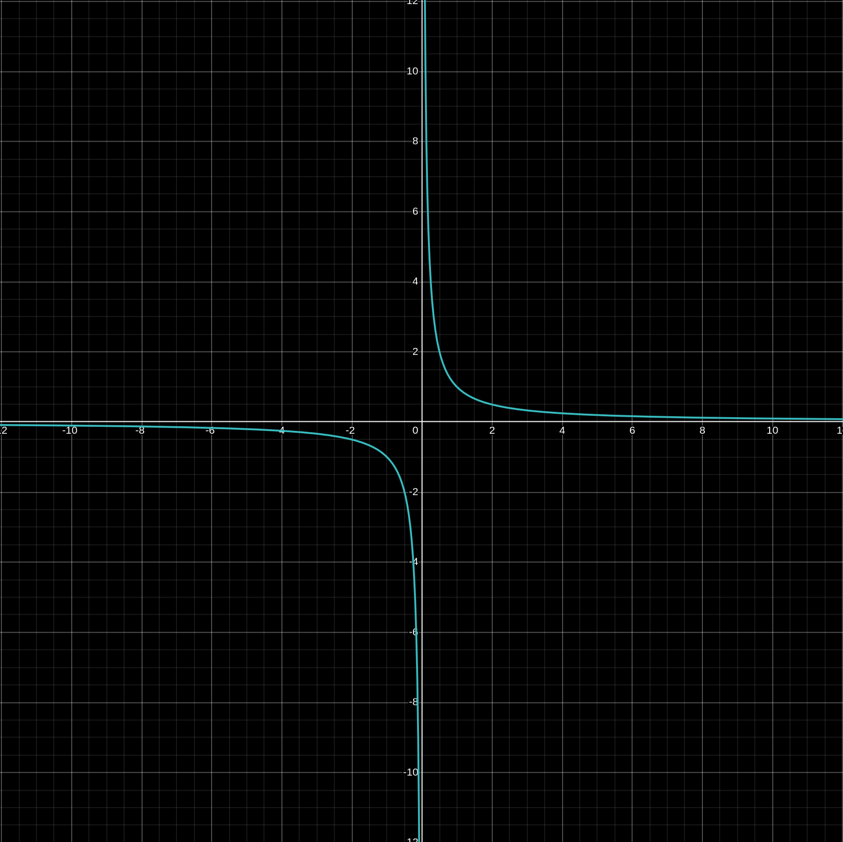
The curve of $\frac{1}{x}$
Let’s revisit the function $\frac{1}{x}$, it has a vertical asymptote at $x = 0$ whereby the curve blows up to $\pm \infty$ from the left and the right side of the vertical asymptote:
\[\begin{align*} \lim\limits_{x\to 0^+} f(x) = \infty \\ \lim\limits_{x\to 0^-}f(x) = -\infty \end{align*}\]The formal one-sided limit definition presented earlier is insufficient to express limits that converges to $\pm \infty$ (i.e. diverge) since $\infty\notin\mathbb{R}$ (i.e. $\mathbb{R}$ contains an infinitely many finite numbers but $\pm\infty$ is not a concrete finite number). Thus we now need a new definition for these limits converging to $\pm\infty$:
$\lim\limits_{x\to a^+} f(x) = \infty$ means ($\forall M \gt 0, \exists \delta \gt 0$ such that $a \lt x \lt a + \delta \implies f(x) \gt M$)
$\lim\limits_{x\to a^-} f(x) = \infty$ means ($\forall M \gt 0, \exists \delta \gt 0$ such that $a - \delta \lt x \lt a \implies f(x) \gt M$)
$\lim\limits_{x\to a} f(x) = \infty$ means ($\forall M \gt 0, \exists \delta \gt 0$ such that $0 \lt |x - a| \lt \delta \implies f(x) \gt M$)
The precise definition for approaching to $-\infty$ is left as exercice (though it’ll be shown in an example shortly). Essentially what the definition states is that regardless of how arbitrary large $M$, we can find a value $x$ within the neighborhood of $a$ (the $\delta$ window) such that $f(x)$ is larger than $M$. In other words, regardless how large $M$ is, there’s always going to be another value larger than it within the neighborhood. Sort of reminds me of the two archmidean properties. Let’s use these precise definition to prove the behavior of $\frac{1}{x}$:
Example: Show (1) $\lim\limits_{x\to 0^+} f(x) = \infty$ and (2) $\lim\limits_{x\to 0^-}f(x) = -\infty$
Rough Work for (1): Given $M \gt 0$, we want to define a $\delta \gt 0$ such that $0 \lt x \lt 0 + \delta \implies f(x) = \frac{1}{x} \gt M$. Thus we want the following:
\[\begin{align*} 0 \lt x \lt \delta &\implies \frac{1}{x} \gt M \\ &\implies x \lt \frac{1}{M} \\ &\implies x \lt \delta \lt \frac{1}{M} \end{align*}\]So take $\delta = \frac{1}{M}$
Rough Work for (2): Given $M \lt 0$, we want to define a $\delta \gt 0$ such that $0 - \delta \lt x \lt 0 \implies f(x) = \frac{1}{x} \lt M$. Let’s recall the following:
- $x \lt 0$ so let’s define $x’ \gt 0$ such that $x = -x’$
- $M \lt 0$ so let’s define $M’ \gt 0$ such that $M = -M’$
- $-\delta \lt -x’ \lt 0 \implies 0 \lt \boxed{x’ \lt \delta}$
When approaching $+\infty$, we want $f(x)$ to exceed $M$ so we need $x$ to be small. But when we approach $-\infty$, we want $f(x)$ to go below $M$, so the inequalities are reversed. This could explain any unease you may had when working on the proof for (2). Thus we shall take $0 \lt \delta = \frac{1}{M’} = \frac{-1}{M}$ where $M < 0$ (i.e. negative). While I try not to give a complete proof as this is an accompanying material to the course and not a replacement, I think the rough work will make more sense when seeing it in proven formally:
Let $M \lt 0$ and choose $0 \lt \delta = \frac{-1}{M}$. Then $0 - \delta \lt x \lt 0 \implies -\delta \lt x \implies -(-\frac{1}{M}) \lt x \implies \frac{1}{x} \lt M$ as required. (i.e. we need to show that for any $M \lt 0$, for all $x$ in the neighborhood of 0 (from the left), $f(x)$ will be less than $M$). Therefore $\lim\limits_{x\to 0^-}f(x) = -\infty$.
Observe how our favorite function thus far, $\frac{1}{x}$, exhibits another convergence, but this time to a finite value 0 in what appears to be another asymptote called the horizontal asymptote. Thus far we have discussed the precise definition of what it means to converge to a point from the left and the right as the curve approaches to a particular point in the cartesian plane to either a finite value or to $\pm \infty$. Yet, we still lack the language to describe limits as $x$ approaches to $\pm \infty$. Thus here are the last missing pieces:
Limit Definitions @ $\pm\infty$: $\lim_{x\to\infty} f(x) = L$ where $L$ could be $\pm \infty$ or $L\in\mathbb{R}$
- If $L\in\mathbb{R}$: $\forall\epsilon \gt 0$, $\exists \alpha\in\mathbb{R}$ such that $(x \gt \alpha)\implies |f(x)-L|\lt\epsilon$
- If $L = \infty$: $\forall M \gt 0$, $\exists \alpha\in\mathbb{R}$ such that $(x \gt \alpha)\implies f(x)\gt M$
- If $L = -\infty$: $\forall M \lt 0$, $\exists \alpha\in\mathbb{R}$ such that $(x \gt \alpha)\implies f(x)\lt M$
As usual, the precise definitions for $\lim\limits_{x\to -\infty} f(x) = L$ is left as an exercise to the readers. Suppose we have a sequence $(x_n) \to a$, would the limit $\lim\limits_{x\to a} f(x) = \lim\limits_{n\to\infty} f(x_n)$? That is what the next theorem is about:
Theorem: Let $f$ be defined on a set $S$ and let $a$ be the limit of some sequence in $S$ (including the possibility that $a = \pm\infty$). Let $L\in\mathbb{R}$. Then:
$\lim\limits_{x\to a}f(x) = L \iff $ for every sequence $(x_n)$ in $S$ with limit $a$ but $x_n \ne a \forall n$, we have $\lim\limits_{n\to\infty}f(x_n) = L$
Let’s revisit the limit laws again but for functions instead of sequences:
LIMIT LAWS: let $f, g$ be functions defined on a set $S$ for which $\lim\limits_{x\to a}f(x) = L, \lim\limits_{x\to a}g(x) = M$ for $L, M$:
- $\lim\limits_{x\to a}(f(x) + g(x)) = L + M$
- $\lim\limits_{x\to a} (fg)(x) = LM$
- $\lim\limits_{x\to a} (\frac{f}{g})(x) = \frac{L}{M}, \qquad M \ne 0, g\ne 0$ around $a$
Note: the limit laws above apply for one-sided limits as well as for approaching the function to $\pm\infty$ (i.e. $a$ does not need to be a real number).
The limit laws handle sums, products, and quotients. But what about more complex functions? Composite functions are necessary to construct any complex functions yet we will soon discover the limit laws do not apply.
\[\begin{align*} f(x) = 1 + x\sin(\frac{\pi}{x}), g(x) = \begin{cases} 4 & ,x \ne 1 \\ -4 & ,x = 1 \end{cases} \end{align*}\]WARNING: Composite functions does not respect the limit laws
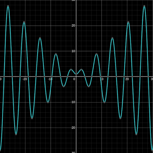
The graph of $1+x\sin(\frac{\pi}{x})$
Let $x_n = \frac{2}{n}$ for $n\in\mathbb{N}$ and $\lim\limits_{n\to\infty}x_n = 0$.
When n is even, $f(x_n) = 1 + x_n \sin(\frac{\pi}{x_n}) = 1 + \frac{2}{n}\sin(\frac{\pi}{\frac{2}{n}}) = 1 + \boxed{\frac{2}{n}\sin(\frac{n\pi}{2})} = 1 + \boxed{0} = 1$
When n is odd, $f(x_n) = 1 + x_n \sin(\frac{\pi}{x_n}) = 1 + \frac{2}{n}\sin(\frac{\pi}{\frac{2}{n}}) = 1 + \boxed{\frac{2}{n}\sin(\frac{n\pi}{2})} = 1 + \boxed{\pm \frac{2}{n}} \ne 1$
Hence the composition is: \(\begin{align*} $g\circ f$(x_n) = g(f(x_n)) = \begin{cases} g(1) & \text{$n$ is even} \\ g(1\pm\frac{2}{n}) & \text{$n$ is odd} \end{cases} = \begin{cases} -4& \text{$n$ is even} \\ 4 & \text{$n$ is odd} \end{cases} \end{align*}\)
As $g\circ f(x_n)$ alternates between -4 and 4, $\lim\limits_{n\to\infty}g\circ f(x_n)$ does not exist and thus neither does $\lim\limits_{n\to\infty}g\circ f(x)$
So what can we conclude about the limits for a composite function then? Well there are now two conditions that need to be satisfied instead of one. For the composite function $g\circ f$:
- the inner function $f(x)$ converges to a value that exist in the outer function’s (i.e. $g(x)$) domain (a requirement already for the composite function to exist)
- $g$, the outer function, is continuous on $f(x) = L$ (NEW CONDITION)
Theorem on the Limits of Composite Functions: let $f$ be a function defined on $S$ for which $\lim\limits_{x\to a}f(x) = L$ exists within $L\in\mathbb{R}$. Let $g$ be a function defined on $\{f(x) | x\in S\} \cup \{L\}$ which is continuous at $L$. Then:
$\lim\limits_{x\to a}(g\circ f)(x) = g(L)$ (i.e. $\lim\limits_{x\to a}(g\circ f)(x) = g(\lim\limits_{x\to a}f(x)$)
Here are some facts about the following functions:
- $\lim\limits_{x\to 0} \frac{\sin(x)}{x} = 1$
- $\lim\limits_{x\to 0} \frac{\cos(x) - 1}{x} = 0$
But one may ask how did one came to this conclusion? If we were to approach this problem using what we have seen thus far, it would seem impossible. But you may recall seeing how the squeeze theorem could be utilised to determine whether a difficult sequence converges by bounding it between two simpler sequences. We’ll employ the same idea to determine the limits presented above by bounding these difficult functions between other simpler functions and see what happens.
Squeeze Theorem (for functions): suppose $f(x)\leq g(x)\leq h(x) \forall x$ and $\lim\limits_{x\to a}f(x) = L = \lim\limits_{x \to a} h(x)$ then $\lim\limits_{x \to a} g(x) = L\in\mathbb{R}$
Example: Show $\lim\limits_{x\to 0} \frac{\sin(x)}{x} = 1$
For $\frac{-\pi}{2}\lt x \lt \frac{\pi}{2}$ and $x\ne 0$, we have:
\[\cos x \leq \sin\frac{x}{x} \leq 1 \nonumber\]where:
- $\lim\limits_{x\to 0} g(x) = \lim\limits_{x\to 0} \cos x = \cos(0) = 1$
- $\lim\limits_{x\to 0} h(x) = \lim\limits_{x\to 0} 1 = 1$
So by squeeze theorem, $\lim\limits_{x\to 0} \frac{\sin(x)}{x} = 1$
Note Showing $\lim\limits_{x\to 0} \frac{\cos(x) - 1}{x} = 0$ is more involved but as a hint:
\[\begin{align*} \frac{\cos (x) - 1}{x} &= (\frac{\cos (x) - 1}{x})(\frac{\cos (x) + 1}{\cos (x) + 1}) \\ &= \frac{\cos^2x - 1}{x(\cos x+1)} \\ &= \frac{-\sin^2x}{x(\cos x + 1)} \\ &= -(\frac{\sin x}{x})(\frac{\sin x}{\cos x + 1}) \end{align*}\]DIFFERENTIATION
After many weeks taking a calculus course, we finally have reached the point of learning what most think of calculus: differentiation (and integration). I am not going to delve much into this subject despite being a central component of Calculus simply because it is both a review from Highschool calculus and is not distinct from a regular calculus course itself.
The central theme in the course thus far has been on limits considering how many weeks have been dedicated to the study of limits and its convergence both using the precise definition and the simple definition of what it means to take the limit of a function as it approaches to a finite number or to $\pm\infty$. It turns out unsurprisingly that the definition of a function being differentiable at a particular point is taking the limit of a function $f$ around the point $a$. This is commonly known as determining the rate of change by observing the slope of the tangent:
Differentiation: Let $f$ be a function defined on an open interval containing the point $a$. We say a function $f$ is differentiable at the point $a$ (or has a derivative at $a$) if:
$\lim\limits_{x\to a} \frac{f(x) - f(a)}{x - a}$ exists and is finite
In other words:
$f’(a) = \lim\limits_{x\to a} \frac{f(x) - f(a)}{x - a}$
Setting $x = a + h$, as $x\to a$, we have $h\to 0$, giving the equivalent formulation:
$f’(a) = \lim\limits_{h\to 0} \frac{f(a+h)-f(a)}{h}$
What makes calculus for Mathematic students vs. Engineering is that we do not rely on intuition of what it means to take the “instantaneous rate of change” but build this up using the precise definition using the $\delta-\epsilon$ proofs to have a clear understanding of what it truly means to take the limit.
Using the definition of differentiation, we can derive all sorts of derivative rules that we come to love and memorise:
Differentiation Rules: Let $f,g$ be differentiable at $x = a$ and let $c\in\mathbb{R}$ be a constant. Then $cf, f+g, fg,$ and $\frac{f}{g}, g(a)\ne 0$ are differentiable at $x = a$. Their derivatives are:
- $(cf)’(a) = cf’(a)$
- $(f+g)’(a) = f’(a) + g’(a)$
- $(fg)’(a) = f’(a)g(a) + f(a)g’(a)$
- $(\frac{f}{g})’(a) = \frac{f’(a)g(a) - f(a)g’(a)}{g^2(a)}, \qquad g(a)\ne 0$
- $(g\circ f)’(a) = g’(f(a))f’(a)$
Chain Rule: if $f$ is differentiable at $x = a$ and $g$ is differentiable at $f(a)$, then $g\circ f$ is differentiable at $a$, with $(g\circ f)’(a) = g’(f(a))f’(a)$
One gripe I have with textbooks is that they often don’t present the entire story of the derivatives of transcendental functions such as $\sin x, \cos x, e^x$ causing many students to omit the chain rule.
For instance, here are the derivatives of common transcendental functions:
- $(\sin x)’ = \cos x$
- $(\cos x)’ = -\sin x$
- $(e^x)’ = (e^x)$
The derivatives above assume the argument is simply $x$. The moment you have anything more complex such as $\sin(x^2)$ or $e^{3x}$, the chain rule is mandatory. Thus when I teach students the derivatives of transcendental functions, I ensure I explicitly present the chain rule in their derivatives as follows:
- $(\sin x)’ = (\cos x)x’$
- $(\cos x)’ = (-\sin x)x’$
- $(e^x)’ = (e^x)x’$
- $(a^x)’ = (a^x \ln a)x’$
- $(\ln x)’ = \frac{1}{x}$
- $(tanx)’ = (sec^2x)x’$
Note: $(e^x)’ = (\bcancel{\ln e} e^x)x’ = (e^x)x’$
Example: Take the derivative of $h(x) = e^{\sin(2x)}$
$h(x) = g\circ f(x)$ where:
- $g(x) = e^x$ and $g’(x) = (e^x)x’ = e^x$
- $f(x) = \sin(2x)$ and $f’(x) = \cos(2x)(2x)’ = 2\cos(2x)$
By chain rule: $h’(x) = (g\circ f)’(x) = g’(f(x))f’(x) = e^{2\sin(2x)} \cdot 2\cos(2x) = 2\cos(2x)e^{\sin(2x)}$
An interesting question is whether if a function being continuous implies differentiability. The answer as it turns out is a resounding no.
Example: Is $f(x)$ differentiable at $x = 0$?
The graph of $\|x\|$
To show $f$ is differentiable at $x = 0$, then we want to show $\lim\limits_{x\to 0}\frac{f(x) - f(0)}{x - 0}$ exists. Recall for the limit to exist, it’s left handed and right handed limits must exist.
Right-Sided Limit:
\[\begin{align*} \lim\limits_{x\to 0^+} \frac{|x|}{x} &= \lim\limits_{x\to 0^+} \bcancel{\frac{x}{x}}, \qquad 0^+ \gt 0\\ &= \lim\limits_{x\to 0^+} 1\\ &= 1 \end{align*}\]Left-Sided Limit:
\[\begin{align*} \lim\limits_{x\to 0^-} \frac{|x|}{x} &= \lim\limits_{x\to 0^-} \bcancel{\frac{-x}{x}}, \qquad 0^- \lt 0 \implies |x| = -x\\ &= \lim\limits_{x\to 0^-} -1 \\ &= -1 \end{align*}\]As $\lim\limits_{x\to 0^+} \frac{|x|}{x} \ne \lim\limits_{x\to 0^-} \frac{|x|}{x}$, $\lim\limits_{x\to 0}\frac{f(x) - f(0)}{x - 0}$ does not exist and thus is not differentiable despite being continuous. Thus we can only conclude from one side, that if $f$ is differentiable at $x = a$ then it is continuous but not the other way around.
Theorem: if $f$ is differentiable at $x = a$, then $f$ is continuous at $x = a$
i.e. differentiable at $x = a \implies f$ is continuous at $x = a$ (but not the other way around)
A good tip to determining whether a function is differentiable at a particular point is to see if there are any sharp edges like we see at $x = 0$ in the function $|x|$.
Mean Value Theorem
One common theme you will notice in analysis is a class of theorems that proves the existence of a phenomen but in a more vague manner. For instance, the Intermediate Value Theorem (IVT) tells us that if a value $y$ lies between $f(a)$ and $f(b)$ then there exists at least one value $x$ in between $a$ and $b$ such that $f(x) = y$ (given $f$ is a continuous function). IVT does not tell us precisely what the $x$ value is but rather bounds the value between two points. Another such theorem in the same spirit as IVT is the Rolle’s Theorem which tells us the existence of a local min or max within two points. But first let us review how to know if we obtain a min or max:
Theorem: Let $f$ be defined on an open interval containing $x_o$. Suppose that $f$ attains its max or minimum at $x_o$ and that $f$ is differentiable at $x = x_o$ then $f’(x_o) = 0$
For a continuous and differentiable function to hit its local min or max at $x = x_o$, we must observe absolutely 0 change at that point (i.e. $f’(x_o) = 0$. We will later explore how to graph functions based on its derivatives but it is important to understand that if the derivative at a particular point is not zero, then the graph is experiencing a change and thus has not hit a local min or max.
Recall that to hit a local min, we must have the derivatives $f’(x_o - \delta) \lt f’(x_o) = 0 \lt f’(x_o + \delta)$ or what I call a happy face. i.e. the signs of the derivatives changes from negative to positive.
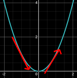
A graph of $x^2$
If I was to draw a table to visualise this change of slope it would look something along the lines of:
\[\begin{array}{c|c} & 0 & \\ \hline - & & + \nonumber \end{array}\]or
\[- \overset{0}{|} + \nonumber\]Now here’s the Rolle’s theorem now that we established the fact that an extremum occurs when the slope is 0 (i.e. $f’(x_o) = 0$.
Rolle’s Theorem: Suppose $f$ is continuous on $[a,b]$, $f$ is differentiable on $(a,b)$ and that $f(a) = f(b)$. Then there exists $c\in(a,b)$ with $f’(c) = 0$
Note: Rolle’s Theorem is actually a special case of the Mean Value Theorem presented below where $f(a) = f(b)$ where by the average rate of change is $\frac{f(b)-f(a)}{b-a} = 0$, so the MVT guarantees there exists some $c$ where $f’(c) = 0$
The next theorem relates to how one can draw a tangent line parallel to the tangent slope which itself does not seem impressive from face value as it states the existence of the average rate between two points is equal to a instantaneous rate of change between the two points:
Mean Value Theorem (MVT): let $f$ be continuous on $[a, b]$ and differentiable on $(a,b)$ then there exists $x\in(a,b)$ with $f’(x) = \frac{f(b)-f(a)}{b-a}$

Illustration of MVT extracted from Paul's Math Notes
While seemingly inconsequential, the consequences of MVT are interesting. For instance, if $\forall x\in\mathbb{R}, f’(x) = 0$ then $f$ is a constant line. But more interestingly is when two functions seemingly have the same slope (i.e. derivative):
Collary of MVT 1: Let $f,g$ be differentiable function on $(a,b)$ and suppose $f’=g’$ on $(a,b)$. Then $\exists c \in\mathbb{R}$ (a constant) such that $f(x) = g(x) + c \forall x$
The strongest corollary of the MVT presented in the course is understanding the behavior of a function based on its slope (derivative):
Collary of MVT 2: Let $f$ be differentiable function on $(a,b)$:
- $f’(x) \gt 0 \forall x\in(a,b) \implies f$ is STRICTLY INCREASING on $(a,b)$
- $f’(x) \lt 0 \forall x\in(a,b) \implies f$ is STRICTLY DECREASING on $(a,b)$
- $f’(x) \geq 0 \forall x\in(a,b) \implies f$ is INCREASING on $(a,b)$
- $f’(x) \leq 0 \forall x\in(a,b) \implies f$ is DECREASING on $(a,b)$
L’Hôpital’s Rule
We have finally made it to the last major topic covered in the course, the L’Hôpital rule, the one rule whose name will reveal whether or not you failed French class (i.e. H is silent in French and as Canadians, we should know at least that much). Thus far in the course, we’ve been working with nice limits whose mathematical results won’t make us scratch our heads. But suppose we have the following limit:
\[\begin{align*} \lim_{x\to a} \frac{f(x)}{g(x)} \end{align*}\]where $a$ can be a one-sided limit, a number or even $\pm \infty$. There are forms where $\lim_{x\to a} f(x)$ and $\lim_{x\to a} g(x)$ could be equal to either $0$ or $\pm \infty$ and would cause our heads to scratch as the results are undefined. These forms are what we call indeterminate forms and there are many such as:
- $\frac{0}{0}$
- $\frac{\infty}{\infty}$
- $0 \cdot \infty$
- $\infty - \infty$
- $0^0$
- $\infty^0$
- $1^\infty$
For instance $\lim\limits_{x\to 0} \frac{\tan (x)}{x} = \frac{0}{0}$ which is undefined.
While some of these forms can be manipulated to be solvable such as in the case of $0\cdot \infty$ where one could rewrite the limit in the form of $\frac{f(x)}{\frac{1}{g(x)}}$ or $0^0$ as $e^{g(x)\ln f(x)}$, others requires another technique:
L’Hôpital’s Rule: let $s$ be one of $a, a^+, a^-, +\infty, -\infty$. Suppose $f,g$ are differentiable functions for which $\lim\limits_{x\to s}\frac{f’(x)}{g’(x)} = L$ exists.
If $\lim\limits_{x\to s} f(x) = \lim\limits_{x\to s} g(x) = 0$ or if $\lim\limits_{x\to s}|g(x)| = \infty$, then $\lim\limits_{x\to s} \frac{f(x)}{g(x)} = L$
To clarify, while there exists indeterminate forms not in rational forms such as $\infty - \infty$, to apply L’Hôpital’s Rule, one must rewrite it into rational form (for $\infty-\infty$ case, you would need to multiply by it’s conjugate and rationalise it).
i.e. indeterminate form $\xrightarrow{\text{rewrite}} \frac{0}{0}$ or $\frac{\infty}{\infty} \xrightarrow{\text{L’Hôpital}} L$
Example: Find $\lim_{x\to 0}\frac{\tan(x)}{x}$
Recall that $\lim\limits_{x\to 0} \tan(x) = \tan(0) = 0$ so we have $\lim\limits_{x\to 0}\frac{\tan(x)}{x} = \frac{0}{0}$ form
As both functions are differentiable around 0 (and $x’ = 1 \ne 0$), we can apply the L’Hôpital Rule: $\lim_{x\to 0}\frac{\tan(x)}{x} = \lim_{x\to 0}\frac{(\tan(x))’}{(x)’ = \lim_{x\to 0}\frac{\sec^2(x)}{1}} = 1$
Example: $\lim_{x\to 0^+} x\ln(x) = 0\cdot \infty$
Recall that $\ln(x)$ and $\frac{1}{x}$ are differentiable around $0^+$ and that $(\frac{1}{x})’ = (x^{-1})’ = -x^{-2} = \frac{-1}{x^2}$ is non-zero for $x\to 0^+$
So we can try L’Hôpital’s rule by rewriting it as a rational function:
\[\begin{align*} \lim_{x\to 0^+} x\ln(x) &= \frac{\ln(x)}{\frac{1}{x}} \to \frac{-\infty}{\infty} \text{form so use L'Hôpital's Rule}\\ &= \frac{(\ln(x))'}{(\frac{1}{x})'}\\ &= \lim_{x\to 0^+} \frac{\frac{1}{x}}{(\frac{-1}{x^2})} \\ &= \lim_{x\to 0^+} -x^2\cdot\frac{1}{x} \\ &= \lim_{x\to 0^+} -x \\ &= 0 \end{align*}\]As stated earlier, one needs to ensure to rewrite the indeterminate form into a rational form such that it is in the form: $\frac{\infty}{\infty}$ or $\frac{0}{0}$. We have seen an example of rewriting $0\cdot \infty$ but let’s now look at rewritting $0^0$ using the fact $e^{\ln(y)} = y, y\gt 0$:
Example: $\lim\limits_{x\to 0^+} x^x$
$x^x$ can be rewritten as $e^{\ln (x^x)} = e^{x\ln (x)}$
Since we know $e^x$ is a continuous function, and is differentiable everywhere. Thus we have:
\[\begin{align*} \lim\limits_{x\to 0^+} x^x &= \lim\limits_{x\to 0^+} e^{\ln(x^x)} \\ &= \lim\limits_{x\to 0^+} e^{x\ln(x)} \\ &= e^{\lim\limits_{x\to 0^+} x\ln(x)} \\ &= e^0, \qquad\text{as shown in the previous example}\\ &= 1 \end{align*}\]Credits:
- MATH1052 Notes from Charles Starling
- Elementary Analysis: The Theory of Calculus by Kenneth A. Ross
Note: I refer to this page as a commentary to the course or an accompanying to the course, these are not class notes. I the author of this page will omit many details and only present the materials and proofs to things I find personally noteworthy and the proofs presented may differ from those listed in the textbook or from the course notes itself.
Note: The reviews are bias and reflects my perception of the course. In addition, the information varies depending on the professor and will likely be outdated.
For More Bias Course Reviews:
- MATH2052 - A Commentary on Calculus and Introductory Analysis 2
- MATH1052 - A Commentary on Calculus and Introductory Analysis 1
- MATH3001 - Real Analysis 1
- MATH1800 - Introduction to Mathematical Reasoning
- MATH2000 - Multivariable Calculus and Fundamentals of Analysis [Fall+Winter]
- PHYS1004 - A Review on Introductory Electromagnetism and Wave Motion
- MATH2107 - Linear Algebra II
- MATH2052 - Calculus and Introductory Analysis II
- PHYS1001 - A Review on Foundations of Physics 1
- MATH1152 - Introductory Algebra 1
- MATH1052 - Calculus and Introductory Analysis 1
- Bias UTM CS Course Review