<?xml version="1.0" encoding="utf-8"?><feed xmlns="http://www.w3.org/2005/Atom" ><generator uri="https://jekyllrb.com/" version="4.4.1">Jekyll</generator><link href="https://randombits.ca/feed.xml" rel="self" type="application/atom+xml" /><link href="https://randombits.ca/" rel="alternate" type="text/html" /><updated>2026-07-15T00:38:13-04:00</updated><id>https://randombits.ca/feed.xml</id><title type="html">RANDOM BITS</title><entry><title type="html">MATH2052 - A Commentary on Calculus and Introductory Analysis 2</title><link href="https://randombits.ca/blog/math2052-commentary" rel="alternate" type="text/html" title="MATH2052 - A Commentary on Calculus and Introductory Analysis 2" /><published>2026-06-11T00:00:00-04:00</published><updated>2026-06-11T00:00:00-04:00</updated><id>https://randombits.ca/blog/math2052-commentary</id><content type="html" xml:base="/blog/math2052-commentary"><![CDATA[<p>This is a commentary to the second introductory course to calculus and analysis which I have a <a href="https://randombits.ca/blog/math2052">course review</a> on if you are interested. The content presented below are from winter 
2022 which may not reflect what is covered in your class today. Furthermore, the information presented will have the author’s own commentary and is <strong>NOT</strong> and should <strong>NOT</strong> be a replacement to attending class. 
The author simply wishes to review the content of the course mixed with their own speculations, views, and emotions as it reflects on the course 5 years later in preparation to their eventual return to 
school after a 2 year break from Mathematics. This course is a follow up on <a href="https://randombits.ca/blog/math1052">MATH1052</a> exploring integrals, different types of convergence such as point-wise and uniform convergence, and 
ends with taylor series and its applications.</p>

<p>As a side note, the commentary presented below heavily resembles Elementary Analysis: The Theory of Calculus by Kenneth A. Ross. This is on purpose as Starling heavily based on the course notes based on this 
textbook.</p>

<p>The course is broken down into 3 main components:</p>
<ol>
  <li><a href="#darboux">Darboux Sums and Integrability</a></li>
  <li><a href="#int-tech">Integration Techniques</a></li>
  <li><a href="#power">Power Series</a></li>
  <li><a href="#taylor">Taylor Series</a></li>
</ol>

<hr />

<p><a name="darboux"></a></p>

<h2 id="darboux-sums-and-integrability">Darboux Sums and Integrability</h2>

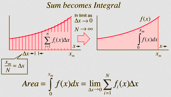
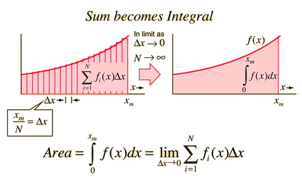
<p>From any regular calculus course, one would know that integration is the process of finding the area under its approximation of the area of a curve using extremely thin and equally-sized rectangles. 
But one can be more formal in how the area is calculated. From elementary school, one learned that to calculate the area of a rectangle by multiplying the length by its width. It turns out we can expand this concept to calculate the area of any curve 
by drawing a series of equally wide rectangles under the curve to approximate the area as seen below:</p>

<div style="background-color: #ffe4c8; width: fit-content; margin: auto">
<img src="/assets/math-physics/courses/math2052/iarea3.png" alt="Approximation of the area of a curve using increasingly narrower rectangles" />
</div>
<p class="caption">Approximation of the area of a curve using increasingly narrower rectangles. Taken from <a href="http://hyperphysics.phy-astr.gsu.edu/hbase/imgmth/iarea3.gif">HyperPhysics</a></p>

<p>Eventually when the width of the rectangles becomes infinitesimally thin, the sum of these infinitesimally thin rectangles gives us the true area under the curve.</p>

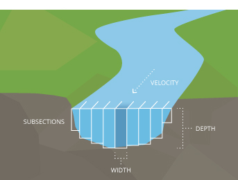
<p>This technique of dividing an interval of a curve with increasingly smaller subintervals resulting in thinner and thinner rectangles to approximate area is not a mere theoretical concept but something that’s actually used in real life. I recall in one of my geography 
courses, the class was sent to a nearby bridge, tasked on measuring the depth of the river at different points, repeating the measurements in smaller partitions to get an approximate area of the 
river.</p>

<p><img src="/assets/math-physics/riverstream_discharge.jpg" alt="" /></p>
<p class="caption">An image I found on google that looked familiar to what I learned in Geography to measure discharge. Source: <a href="https://www.fondriest.com/environmental-measurements/measurements/hydrological-measurements/streamflow-measurements/">Fondriest</a></p>

<p>One question that may arise is how to determine the height of these rectangles as it is clear that these rectangles don’t capture the curves nicely. There are a few ways to determine the height such 
as grabbing the function’s value at the midpoint between each subinterval $[t_i, t_{i+1}]$, the way the author first encountered in their time as a student in computer science. But this choice can feel arbitrary 
with no guarantees whether the height of each subinterval under-estimates or over-estimates the true area. One elegant approach introduced in this course is to consider both cases and see if the two cases 
can reconcile (i.e. be equal to each other) and this approach is called Darboux Sums or Darboux Integrals.</p>

<p>Formally, we define a partition for a function $f$ bounded on $[a,b]$ to be:</p>

<blockquote>
  <p><strong>Partition</strong> of $[a,b]$ is a finite sequence $(t_m)$ with $a = t_0 \lt t_1 \lt t_2 \lt \dots \lt t_n = b$.
Thus $P = \{t_0, t_1, t_2, \dots, t_n\}$</p>

  <p>Put simply, it is a partition is a set of ordered numbers between $a$ and $b$.</p>
</blockquote>

<p>The over-estimated area is called the UPPER darboux sum and the under-estimated rectangles are called the lower darboux sum making use of the definitions of supremum and infimum encountered in the previous 
course. As one can easily imagine, the two darboux sums take the “max” (supremum) and “min” (infimum) of the curve within each subinterval as the height of the rectangles.</p>

<blockquote>
  <p>For a subset $S \subseteq [a, b]$, we let:</p>

  <p>$M(f,S) = sup\{ f(x) : x \in S\}$ i.e. “Max height of each rectangle”</p>

  <p>$m(f,S) = \inf\{ f(x) : x \in S \}$ i.e. “Min height of each rectange”</p>
</blockquote>

<p>Thus we can formally define the upper and lower darboux sums as the following:</p>

<blockquote>
  <p><strong>UPPER Darboux Sum:</strong> $U(f,P) = \sum\limits^n_{k=1} \underbrace{M(f, [t_{k-1}, t_k])}_{\text{height}} \cdot \underbrace{(t_k-t_{k-1})}_{\text{base}}$</p>
</blockquote>

<blockquote>
  <p><strong>LOWER Darboux Sum:</strong> $L(f,P) = \sum\limits^n_{k=1} \underbrace{m(f,[t_{k-1}, t_k])}_{\text{height}}\underbrace{(t_k - t_{k-1})}_{\text{base}}$</p>
</blockquote>

<p>Recall the objective is to approximate and eventually get the true area under the curve by taking the sum of the area of extremely thin rectangles. Also recall that the area of a rectangle is simply 
width multiplied by its height.</p>

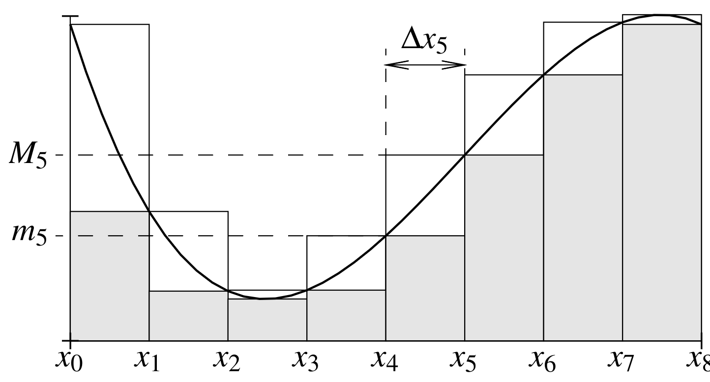
<p><img src="/assets/math-physics/courses/math2052/darboux-sums.png" alt="A sample of darboux sums" width="750px" /></p>
<p class="caption">A sample of darboux sum where the lower sum is the area of the shaded rectangles and the upper sum is the area of the entire rectangles (shaded + unshaded regions). Taken from 
<a href="https://ocw.mit.edu/courses/18-100a-real-analysis-fall-2020/mit18_100af20_basic_analysis.pdf">MIT OCW Real Analysis notes</a></p>

<p>One may see the upper and lower darboux sums reformulated as the following:</p>

<blockquote>
  <p><strong>Upper Darboux Sum:</strong> $U(f,P) = \sum\limits^n_{k=1} M_i\Delta x_i$</p>

  <p><strong>Lower Darboux Sum:</strong> $L(f,P) = \sum\limits^n_{k=1} m_i \Delta x_i$</p>

  <p>where:</p>

  <p>$M_i = \sup\{f(x): x_{i-1} \leq x \leq x_i \}$</p>

  <p>$m_i = \inf\{f(x): x_{i-1} \leq x \leq x_i \}$</p>
</blockquote>

<p>Recall in our definition, $f$ is a bounded function on $[a,b]$ so it attains a global min and a global max value. In addition, every partition of $[a,b]$ will contain at least the endpoints $a$ and $b$. 
One key observation is that the local min and max are bounded by the global extremas:</p>

<ul>
  <li>$M(f, [t_{k-1},t_k]) \leq M(f,[a,b]) = M$</li>
  <li>$m(f, [t_{k-1}, t_k]) \geq m(f, [a,b]) = m$</li>
</ul>

<p>where $[t_{k-1},t_k] \subseteq [a,b]$. Intuitively, finer partitions capture the function more accurately, so the underestimate improves and the overestimate tightens (potentially 
decreases). Given this fact, we have the following:</p>

<blockquote>
  <p>$m(b-a) = m(f, [a,b])(b-a) \leq L(f,P) \leq U(f,P) \leq M(f,[a,b])(b-a) = M(b-a)$</p>
</blockquote>

<p><strong>Quick Breakdown:</strong></p>

\[\require{cancel}
\begin{align*}
U(f,P) = \sum\limits^n_{k=1} M(f,[t_{k-1},t_k])(t_k - t_{k-1}) &amp;\leq \sum\limits^n_{k=1} M(f,[a,b])(t_k - t_{k-1})\\
&amp;= \underbrace{M(f, [a,b])}_{\text{const}} \sum\limits^n_{k=1} (t_k-t_{k-1}) \\
&amp;= M((\bcancel{t_1} - t_0) + (\bcancel{t_2} - \bcancel{t_1}) + \dots + (\bcancel{t_{n-1}} - \bcancel{t_{n-2}})  + (t_n - \bcancel{t_{n-1}})) \\
&amp;= M(t_n - t_0) \\
&amp;= M(b - a) \\
\therefore U(f,P) \leq M\sum\limits^n_{k=1} (t_k-t_{k-1}) \leq M(b-a)
\end{align*}\]

<p>Similar idea to show $m(f, [a,b])(b-a) \leq L(f,P) \leq U(f,P)$</p>

<p>Since $m(f,[t_{k-1},t_k]) \leq M(f, [t_{k-1}, t_k])$ (since $\inf \leq \sup$ by definition), we have $L(f,P) \leq U(f,P)$ for any single Partition P. (
Note: it is not immediately clear whether $L(f,P_1) \leq U(f.P_2)$ for <strong>different</strong> partitions $P_1,P_2$, a question we will address shortly.)</p>

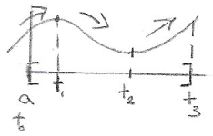
<p><img src="/assets/math-physics/courses/math2052/darboux-sums-under-over.png" alt="Hand-written Illustration of L(f) and U(f)" width="750" /></p>

<p>Given this proposition, we see these darboux sums are bounded and by consequence are guaranteed of the existence of an upper Darboux Integral $U(f)$ and lower Integral $L(f)$:</p>

<blockquote>
  <p><strong>Upper Darboux Integral:</strong> $U(f) = \inf\{U(f,P) : P$ is a partition of $[a,b]$ $\}$. Often represented as $\overline{\int}_a^b f(x)dx$</p>

  <p><strong>Lower Darboux Integral:</strong> $L(f) = \sup\{L(f,P): P$ is a partition of $[a,b]$ $\}$. Often represented as $\underline{\int}_a^b f(x)dx$</p>
</blockquote>

<p>Similar to how a limit exists if the LHS and RHS limits exist, we say $f$ is <strong>INTEGRABLE</strong> on $[a,b]$ if $U(f) = L(f)$ or $\overline{\int} a^b f(x)dx = \underline{\int}_a^b f(x)dx$</p>

<blockquote>
  <p><strong>Darboux Integral:</strong> f is <strong>INTEGRABLE</strong> on $[a,b]$ if $U(f)=L(f)$. Often represented as $U(f)=L(f)=\int\limits_a^b f(x)dx$</p>
</blockquote>

<p>where $f(x)$ can be seen as the height and $dx$ as the width of the rectangle approaching to 0.</p>

<p>Showing whether a function is integrable is a lot of work and thus will be omitted. Please read Ross Analysis or search online for an example. However, what I will show and find more interesting is to 
show a function $f$ this <strong>NOT</strong> integrable. In Engineering, we are always given ‘‘nice” functions that always have integrals but it turns out there are functions that don’t have an “area”. One 
potential example is comparing the area between two functions that appear to be the same but one has finite number of holes and the other has infinitely many holes in the graph. One is integrable 
and the other is not.</p>

<p><strong>Example:</strong></p>

<p>\(f(x) = \begin{cases} 
      1 &amp; x \in \mathbb{Q} \\
      0 &amp; x \notin \mathbb{Q} 
\end{cases}\) on $[a,b]$. Show that f is not integrable.</p>

<p>Note that every interval $[t_{k-1}, t_k]$ contains a rational and irrational number (i.e. by the density of $\mathbb{Q}$)</p>

<p>We have:
\(\begin{align*}
M(f, [t_{k-1},t_k]) = 1 \forall k &amp;\implies U(f,P)=1(b-a) = (b-a) &amp;&amp;\implies U(f) = b-a \\
m(f, [t_{k-1},t_k]) = 0 \forall k &amp;\implies L(f,P)=0(b-a) = 0 &amp;&amp;\implies L(f) = 0
\end{align*}\)</p>

<p>Thus $U(f) \ne L(f)$ and by definition, $f$ is not integrable on $[a,b]$</p>

<p>Any engineering student should be surprised of this result, especially on the idea that one can be asked to determine if a function is integrable or not. This is one of many examples that differentiates 
between Math and Engineering students. Math students are expected to not take anything for granted unless told otherwise (reality is that there are some materials that are just too complex at the moment 
to learn).</p>

<p>Previously, we saw that for any partition $P, U(f, P) \leq  U(f,[a,b])$. We previously reasoned that a finer partition does a much more accurate job in capturing the function’s true behavior. Geometrically, 
we are summing more thinner rectangles whose lower and upper values $M_i$ and $m_i$ are tighter to the true value. Thus we can generalise the following:</p>

<blockquote>
  <p><strong>Lemma 1:</strong> Let $f$ be bounded function on $[a,b]$. If $P,Q$ are partitions of $[a,b]$ with $P\subseteq Q$ (i.e. $Q$ is a “finer” partition within $[a,b]$ / has more points in the partition). Then:</p>

  <p>$L(f,P) \leq L(f,Q) \leq U(f,Q) \leq U(f,P)$</p>
</blockquote>

<p>Essentially the lemma is stating that adding points to the partition <strong>decreases</strong> the upper sum and <strong>increases</strong> the lower darboux sum. Geometrically, this would correspond to having more thinner 
rectangles to approximate the area more accurately.</p>

<p>Similarly, we can now make the claim that for any partition, the lower darboux sum will always be less than (or equal to) any upper darboux sum regardless of the partition.</p>

<blockquote>
  <p><strong>Lemma 2:</strong> Let $f$ be bounded on $[a,b]$ and let $P,Q$ be partitions of $[a,b]$. Then $L(f,P) \leq U(f,Q)$</p>
</blockquote>

<p><strong>Proof:</strong> Consider the partition $P \cup Q$. Note that we know nothing about the partitions $P$ and $Q$ but we do know we can construct a larger partition $P\cup Q$ such that:</p>
<ul>
  <li>$P\subseteq P \cup Q$</li>
  <li>$Q\subseteq P \cup Q$</li>
</ul>

<p>So by the previous lemma (lemma 1),</p>
<ul>
  <li>$L(f,P) \leq L(f, P \cup Q)$ (i.e. adding points to the partition increases the lower darboux sum)</li>
  <li>$U(f,P\cup Q) \leq U(f,Q)$ (i.e. adding points to the partition decreases upper darboux sum)</li>
</ul>

<p>Chaining these two conclusion, we have: $L(f,P) \leq L(f, P \cup Q) \leq U(f,P\cup Q) \leq U(f,Q)$</p>

<p>Thus lemma 2 tells us tht any any lower sum is below any upper sum. But the supremum and infimum are the tightest bounds we can get. What does lemma 2 tells us about these bounds?</p>

<blockquote>
  <p><strong>Lemma 3:</strong> Let $f$ be bounded on [a,b]. Then $L(f) \leq U(f)$</p>
</blockquote>

<p>Previously in lemma 2, we proved that regardless of the partition, the upper darboux sum is always greater (or equal to) the lower darboux sum. 
This is an extension of the previous lemma but even stronger by tighting the bound such that even the GREATEST lower darboux sum is less than the LEAST upper darboux sum.</p>

<p>By the definition of Darboux Integrals, we know that a function is integrable if its lower and upper sum are equal (i.e. $L(f) = U(f)$). However, this definition requires us to verify this equality 
directly which at times can be difficult due to $U(f)$ and $L(f)$ being defined as the infima and suprema of the upper and darboux sums of an infinitely many bounded finite-partitions respectively. 
One can use the following characterisation to determine if a function is integrable:</p>

<blockquote>
  <p><strong>Theorem 1 (Cauchy Criterion):</strong> a bounded function $f$ on $[a,b]$ is integrable $\iff \forall \epsilon &gt; 0 \exists$ a partition $P$ of $[a,b]$ such that $U(f,P) - L(f,P) \lt \epsilon$</p>
</blockquote>

<p>As one may recall from the <a href="../math1052-commentary">previous course</a>: For any $\epsilon &gt; 0$, if the difference between two values is less than every positive $\epsilon$ then the difference must be 0.</p>

\[\text{for any two real numbers } x, x_o, \text{ if } |x-x_o| \lt \epsilon, \forall \epsilon \gt 0 \nonumber \\
\text{then }x = x_o\]

<p>A common example is the value $1.\overline{9} = 1.9999\dots$ (i.e. the 9 repeats infinitely many times).</p>

<p>No matter what $\epsilon \gt 0$ you choose, we have $2 - 1.\overline{9} \lt \epsilon$</p>

<p>For instance:</p>
<ul>
  <li>$|2 - 1.9| &lt; 0.1$</li>
  <li>$|2 - 1.99| &lt; 0.01$</li>
  <li>$|2 - 1.999| &lt; 0.001$</li>
</ul>

<p>As we add more 9s, the difference gets smaller. In this limit, the difference converges to 0. Thus $2 - 1.\overline{9} = 0$ or $1.\overline{9} = 2$.</p>

<p>Many integration problems found in Engineering have one thing in common, they tend to be continuous? Is there a particular reason for this? It turns out that it is easy to create integration 
problems as long as the functions are continuous:</p>

<blockquote>
  <p><strong>Theorem 2:</strong> Every continuous function $f$ on $[a,b]$ is integrable</p>
</blockquote>

<p>However, sometimes a student can be blessed or cursed (depending on perspective) with a piecewise function. But in particular, these discontinuous functions tend to have one thing in common, 
they are montonic functions. Recall that a monotone function is a function that is either increasing or decreasing (not strictly) and do not have to be continuous. For instance, take a piecewise 
montonic function, the step function that jumps upward at finitely many points but never decreases. Professors don’t pose students integration problems out of nowhere, 
they rely on the next theorem to pose piecewise functions to students:</p>

<blockquote>
  <p><strong>Theorem 3:</strong> Every monotone functions on $[a,b]$ is integrable</p>
</blockquote>

<p>The next set of facts will be given without any commentary:</p>
<blockquote>
  <p>let $f,g$ be integrable on $[a,b]$ and let $c\in\mathbb{R}$. Then:</p>
  <ol>
    <li>$cf$ is integrable with $\int^b_a cf = c\int^b_a f$ (scalar multiplication)</li>
    <li>f+g is integrable with $\int_a^b (f + g) = \int_a^b f + \int_a^b g$ (additivity)</li>
    <li>if $f(x) \leq g(x) \forall x\in [a,b]$ then $\int_a^b f(x)dx \leq \int_a^b g(x)dx$ (monotonicity)</li>
    <li>if $g$ is a continuous non-negative function and  $\int_a^b g(x)dx = 0$ then $g(x) = 0 \forall x\in [a,b]$</li>
    <li>let $a \lt c \lt b$ and if $f$ is integrable on $[a,c]$ and on $[c,b]$ then $\int_a^b f = \int_a^c + \int_c^b$ (additivity of intervals)</li>
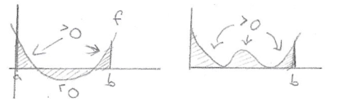
    <li>$|f|$ is integrable on $[a,b]$ and $|\int_a^b f| \leq  \int_a^b |f|$ (triangle inequality)
<img src="/assets/math-physics/courses/math2052/integration-abs.png" alt="Visual illustration of the difference between taking absolute val of an integral v.s taking the integration of a abs(f)" /></li>
  </ol>
  <p class="caption">Illustration of $\|\int_a^b f\|$ on the left and $\int_a^b \|f\|$ on the right</p>
</blockquote>

<p>Previously, we stated that if $f$ is either montone or continuous, then it is integrable. But not all functions are monotone nor continuous which could severely restrict what types of curves we can 
compute the area under. But what if we broke the functions into separate individual pieces? That is what piecewise functions attempt to do and we shall be exploring further the integrability of 
such functions.</p>

<blockquote>
  <p><strong>Piecewise Monotone:</strong> $f$ is called <strong>piecewise monotone</strong> on $[a,b]$ if there is a partition $P$ of $[a,b]$ such that $f$ is monotone on each open subinterval $(t_{k-1},t_k)$.</p>
</blockquote>

<p><img src="/assets/math-physics/courses/math2052/piecewise-monotone.png" alt="Illustation of a piecewise monotone function" /></p>
<p class="caption">A piecewise monotone function</p>

<blockquote>
  <p><strong>Piecewise Continuous:</strong> $f$ is called <strong>piecewise continuous</strong> on $[a,b]$ if there is a partition $P$ of $[a,b]$ such that $f$ is uniformly continuous on each open subinterval $(t_{k-1},t_k)$</p>
</blockquote>

<p><img src="/assets/math-physics/courses/math2052/piecewise-cts.png" alt="Illustation of a piecewise monotone function" /></p>
<p class="caption">A piecewise continuous function</p>

<blockquote>
  <p><strong>Theorem 4:</strong> If $f$ is <strong>piecewise continuous</strong> or <strong>(bounded) piecewise monotone</strong> on $[a,b]$, then it is integrable on $[a,b]$</p>
</blockquote>

<p>With theorem 4, we have now covered the integrability of nearly all functions encountered in engineering and applied mathematics (at least at a freshman level).</p>

<p>Now we have covered enough to discuss the one of the biggest theorem in calculus: the fundamental theorem of calculus (FTC). Specifically we will cover the first part of FTC but essentially 
the fundamental theorem of calculus connects differentiation covered in the previous course with integration to show they are roughly inverses of each other. In addition, it also teaches us how to 
compute the integral of a function much more efficiently (at least by hand).</p>

<blockquote>
  <p><strong>Theorem 5 (Fundamental Theorem of Calculus 1):</strong> if $f$ is continuous on $[a,b]$ and differentiable on $(a,b)$ and if $f’$ is integrable on $[a,b]$,
then $\underbrace{\int_a^b f’(x)dx}_{\text{sum of infinitesimal changes}} = \underbrace{f(b)-f(a)}_{\text{total change}}$</p>
</blockquote>

<p>The first part of the theorem tells us that integrating a derivative gives us the original function’s change. Recall that the derivative $f’(x)$ tells us the rate of change of the function $f$ at 
each point. Summing (i.e. integrating) all these infinitesimal changes from $a$ to $b$ should give the total change $f(b) - f(a)$.</p>

<p>Thus, by the fundamental theorem of calculus part 1, we have a practical method to compute definite integrals. Instead of constructing darboux sums, we can use antiderivatives.</p>

<p>You may see the term definite and indefinite integrals thrown around, essentially one specifies its bound and the other does not. But here’s a more complete definition:</p>
<ul>
  <li><strong>Definite Integral:</strong> the integral has bounds $[a,b]$ and evaluates to a single real number</li>
  <li><strong>Indefinite Integral:</strong> the integral has no bounds and represents a family of antiderivatives $F(x) + C$ where $C\in\mathbb{R}$</li>
</ul>

<p>Suppose $a \lt b$, then what would it mean if we switch the bounds around? (i.e. $\int_b^a f(x)dx$?). By the fundamental theorem of calculus part 1, we have:</p>

\[\int_a^b f(x)dx = F(b) - F(a) \nonumber\]

<p>So if we were to swap the bounds, we would have: $\int_b^a f(x)dx = F(a) - F(b) = - (F(b) - F(a)) = - \int_a^b f(x)dx$</p>

<blockquote>
  <p>If $a \lt b$ then $\int_b^a f(x)dx = - \int_a^b f(x)dx$</p>
</blockquote>

<p>If $F$ is an antiderivative of $f$ (i.e. $F’ = f$), then:</p>

\[\int_a^b f(x)dx = F(x)|_a^b = F(b) - F(a) \nonumber\]

<p>As a consequence, we also have the following (the second part of the FTC):</p>

\[\frac{d}{dx}\int f(x)dx = f(x) \nonumber\]

<p>While FTC 1 lets us compute definite integrals using antiderivatives, FTC 2 guarantees that the antiderivatives exist.</p>

<blockquote>
  <p><strong>Theorem 6 (Fundamental Theorem of Calculus 2):</strong> let $f$ be integrable on $[a,b]$ and let $F(x) = \int_a^x f(t)dt$. Then $F$ is continuous on $[a,b]$. Moreover, 
if $f$ is continuous at $x_o\in(a,b)$ then $F$ is differentiable at $x_o$, thus $F’(x_o) = f(x_o)$.</p>

  <p>This is a complicated way of saying the derivative undoes the integration: $\frac{d}{dx}\int f(x)dx = f(x)$</p>
</blockquote>

<p><strong>Connection to Theorem 2:</strong> Recall from Theorem 2 that every continuous function on [a,b] is integrable. By FTC 2, we not have an explicit statement that every continuous function has an antiderivative.</p>

<p>On the same subject, it is important to note that even if an antiderivative exists, it does <strong>NOT</strong> mean it is integrable. There is a strong reason for why the formal definition of the FTC 2 requires 
$f$ to be continuous (or at least integrable). Having an antiderivative is not enough.</p>

<p><strong>Example:</strong></p>

\[F(x) = \begin{cases} 
      x^2\sin(\frac{1}{x}) &amp; x \neq 0 \\ \nonumber
      0 &amp; x = 0
\end{cases}\]

<p>$F(x)$ is differentiable everywhere but <strong>DIFFERENTIABILITY $\bcancel{\implies}$ Integrability</strong></p>

<p>For $x \neq 0, f(x) = F’(x) = 2x\sin(\frac{1}{x}) + x^2(\cos(\frac{1}{x}))(\frac{-1}{x^2}) = 2x\sin(\frac{1}{x}) - \cos(\frac{1}{x})$</p>

<p>As $x\to 0$, it widly oscillates between 1 and -1 according to Wikipedia and thus is discontinuous around the neighborhood $x = 0$. With some math I won’t get into, this function apparently broke 
the accepted knowledge of what functions were differentiable everywhere and its derivative was bounded, the derivative was always integrable. As this is a first-year course in Calculus, 
we are strictly referring Integrability as Riemann/Darboux integrable. Using the definitions presented in the blog, this function is not Darboux Integrable.</p>

<hr />

<p><a name="int-tech"></a></p>

<h2 id="integration-techniques">Integration Techniques</h2>

<p>Thus far we have covered what it means to take an integral of a function and what sorts of functions are integrable. Let us now use the fundamental theorem of calculus part 1 and various integration 
techniques to compute integrals.</p>

<p>Here are some basic integration rules to know:</p>

<ul>
  <li><strong>constant:</strong> $\int a dx = ax + C, a\in\mathbb{R}$</li>
  <li><strong>power rule:</strong> $\int x^n dx = \frac{x^{n+1}}{n+1} + C, n\neq -1$</li>
  <li><strong>reciprocal:</strong> $\int \frac{1}{x}dx = \ln |x| + C$</li>
  <li><strong>sum/difference:</strong> $\int [f(x) \pm g(x)]dx = \int f(x)dx \pm \int g(x)dx$</li>
</ul>

<p><strong>Exponential and Logarithmic Functions:</strong></p>
<ul>
  <li>$\int e^x dx = e^x + C$</li>
  <li>$\int a^x dx = \frac{a^x}{\ln(a)} + C, a \gt 0, a\neq 1$</li>
  <li>$\int \ln(x) dx = x\ln(x) - x + C$</li>
  <li>$\int \frac{1}{x\ln (x)} dx = \ln |\ln(x)| + C$</li>
</ul>

<p><strong>Trigonometric Functions:</strong></p>
<ul>
  <li>$\int \cos(x) dx = \sin(x) + C$</li>
  <li>$\int \sin(x) dx = -\cos(x) + C$</li>
  <li>$\int \sec^2(x)dx = \tan(x)+C$</li>
  <li>$\int \sec(x)\tan(x)dx = \sec(x) + C$</li>
  <li>And many more …</li>
</ul>

<p>The issue with computing integrals is that it tends to be an exercise of memorisation and practice to know what techniques to use and what the anti-derivatives are. Hence why I don’t find this section 
particular interesting. But nonethless, it is important to go through different common integration techniques one needs to know to survive their calculus course.</p>

<p>Most functions have no anti-derivatives, and thus Mathematicians have discovered or invented techniques to tackle each problem. Before the release of LLMs, integration calculators were notorious for 
giving complicated solutions to integral problems as they often employed their own common generic integration techniques to solve the problem which weren’t student friendly solutions.</p>

<p>The most basic and fundamental integration technique is <strong>substitution</strong> which is essential to understand. It is the most fundamental integration technique that gets employed in many other 
integration techniques so it is primordial to master it.</p>

<blockquote>
  <p><strong>Substitution Rule:</strong> $\int_a^b f(g(x))g’(x)dx = \int_{u(a)}^{u(b)} f(u)du, $ where $u = g(x)$</p>
</blockquote>

<p>The substitution rule works by recognising composite functions. When you see an integrand with “chain rule” structure, you can often times simplify by substituting the problem to an easier integral.
This looks more daunting than it should be so let’s look at a simple example:</p>

<p><strong>Example:</strong> $\int_0^1 e^{2x} dx$</p>

<p>The integrand $e^{2x}$ is composite: $f(x) = e^x$ and $g(x)$ = 2x, so $f(g(x)) = e^{2x}$.</p>

<p>Our basic rule $\int e^x dx = e^x + C$ does not directly apply because of the coefficient 2 on $x$. This is where substitution helps:</p>

<p>Let $u = 2x$. Then:</p>

\[\begin{align*}
u = 2x, \qquad \frac{du}{dx} &amp;= 2\\
dx &amp;= \frac{du}{2}
\end{align*}\]

<p>Thus we can rewrite the integral as:</p>

\[\begin{align*}
\int e^{2x} dx = \int e^u \frac{du}{2} = \frac{1}{2}\int e^u du
\end{align*}\]

<p>The integrand now is in the correct form and thus is solvable.</p>

\[\begin{align*}
\frac{1}{2}\int e^u du = \frac{1}{2} e^u + C
\end{align*}\]

<p>However, as the question posed a definite integral, we must account for the bounds? There are two approaches:</p>

<ol>
  <li>
    <p><strong>Change of Bounds</strong> Determine what the lower and upper bounds are by computing $u(a)$ and $u(b)$ are</p>

\[x = 0: u(0) = 2(0) = 0 \\ \nonumber
 x = 1: u(1) = 2(1) = 2 \nonumber\]

    <p>So now we can integrate directly:</p>

\[\begin{align*}
 \frac{1}{2}\int_0^2 e^u du &amp;= \frac{1}{2} e^u|_0^2 \\
 &amp;= \frac{1}{2}[e^2 - e^0] \\
 &amp;= \frac{e^2 - 1}{2}
 \end{align*}\]

    <p>The benefit with this approach is that we can work entirely in terms of $u$, there is no need to substitute back</p>
  </li>
  <li>
    <p><strong>Substitute Back:</strong> Solve the indefinite integral first, then substitute back $u = 2x$ before evaluating bounds:</p>

\[\begin{align*}
 \int_0^1 e^{2x}dx &amp;= \frac{1}{2}\int_{x=0}^{x=1} e^u du\\
 &amp;= \frac{1}{2} e^u|_{x=0}^{x=1} \\
 \end{align*}\]

    <p>As the bounds are respect to $x$, let’s substitute back our original function $u = 2x$</p>

\[\begin{align*}
 \frac{1}{2} e^u|_{x=0}^{x=1} &amp;= \frac{1}{2}e^{2x}|_0^1 \\
 &amp;= \frac{1}{2}[e^{2(1)} - e^{2(0)}] \\
 &amp;= \frac{e^2 - e^0}{2} \\
 &amp;= \frac{e^2 - 1}{2}
 \end{align*}\]
  </li>
</ol>

<p>I always stress to my students to verify their work if feasible (i.e. if time permits and isn’t overly complex to do so) by taking the derivative of their indefinite integral and see if it matches 
the original integrand:</p>

\[\begin{align*}
(\frac{e^u}{2} + C)' &amp;= \left(\frac{e^u}{2}\right)(u') \\
&amp;= (\frac{e^{2x}}{2})(2x)' \\
&amp;= (\frac{e^{2x}}{\bcancel{2}})(\bcancel{2}) \\
&amp;= \boxed{e^{2x}}
\end{align*}\]

<p>This matches our original integrand $e^{2x}$, so we can be confident our integration is correct.</p>

<p>This verification step catches algebraic errors, wrong coefficients, and misapplied rules. If your derivative doesn’t match the integrand, you have made a mistake somewhere.</p>

<p>The Substitution rule has various names including u-subitution rule or change of variables but the most important thing to take from this rule is its ability to simplify the integrand and it can 
potentially achieve this by cancelling a term due to the derivative of $u$.</p>

<p><strong>Example:</strong></p>

<p>For instance, consider the following problem: $\int \frac{x}{x^2+1}dx$</p>

<p>This problem looks very complicated but if we let $u = x^2+1$ then:</p>

\[\begin{align*}
u = x^2+1 \implies \frac{du}{dx} &amp;= 2x\\
\frac{du}{2x} &amp;= dx
\end{align*}\]

<p>Resulting in the following:</p>

\[\begin{align*}
\int \frac{x}{x^2+1}dx &amp;= \int \frac{\bcancel{x}}{u}\left(\frac{du}{2\bcancel{x}}\right)\\
&amp;= \frac{1}{2} \int \frac{1}{u}du \\
&amp;= \frac{1}{2} \ln(u) \\
&amp;= \boxed{\frac{1}{2} \ln(x^2+1)}
\end{align*}\]

<p><strong>Check:</strong></p>

\[\begin{align*}
\frac{1}{2} (\ln(x^2+1) &amp;= \frac{1}{2} \frac{1}{x^2+1} (x^2+1)') \\
&amp;= \frac{1}{\bcancel{2}} \left(\frac{1}{x^2+1}\right)(\bcancel{2}x) \\
&amp;= \boxed{\frac{x}{x^2+1}}
\end{align*}\]

<p>The next integration technique is called <strong>Integration By Parts</strong>, useful when the integrand is a product of two separate functions where one becomes simpler when differentiated:</p>

<blockquote>
  <p><strong>Integration By Parts:</strong> $\int uv’dx = uv - \int vdu$</p>
</blockquote>

<p><strong>Example:</strong> $\int x\sin(x) dx$</p>

<p>The integrand is a product of two functions $x$ and $\sin(x)$.</p>

<p>Choosing which function is to be $u$ or $v’$ takes practice but in general, I like to always default choosing $u$ to be a polynomial function like the linear function $x$ if applicable, 
else consider whose integral (antiderivative) is the least difficult. According to <a href="https://en.wikipedia.org/wiki/Integration_by_parts">Wikipedia</a>, there is the <strong>LIATE</strong> rule, a rule 
I never heard of till now. This rule is a general guide to choosing the $u$:</p>

<ol>
  <li><strong>L</strong> Logarithmic functions</li>
  <li><strong>I</strong> Inverse Trigonometric Functions: $\arctan(x), \text{arcsec}(x)$, etc.</li>
  <li><strong>A</strong> algebraic functions such as polynomials</li>
  <li><strong>T:</strong> trigonmetric functions: $\sin(x), \tan(x)$, etc.</li>
  <li><strong>E:</strong> Exponential functions</li>
</ol>

<p>Based on my personal experience and this rule, choose $u = x$ and $v’ = \sin(x)$. Thus we have:</p>

\[\begin{align*}
u &amp;= x \qquad v' = \sin(x) \\
\frac{du}{dx} &amp;= 1 \qquad v \ = -\cos(x)
\end{align*}\]

<p>Apply the integration by parts rule, we have:</p>

\[\begin{align*}
\int x\sin(x) dx &amp;= uv - \int vdu\\
&amp;= -x\cos(x) - \int -\cos(x)dx \\
&amp;= -x\cos(x) + \int \cos(x)dx \\
&amp;= \boxed{-x\cos(x) + \sin(x) + C}
\end{align*}\]

<p><strong>Check:</strong> 
\(\begin{align*}
(-x\cos(x) + \sin(x) + C)' &amp;= \bcancel{-\cos(x)} + (\bcancel{-}x)(\bcancel{-}\sin(x)) + \bcancel{\cos(x)} + 0 \\
&amp;= \boxed{x\sin(x)}
\end{align*}\)</p>

<p>One trick to recall the rule is to start with the product rule and get the left side to be in the form $uv’$:</p>

\[\begin{align*}
(uv)' &amp;= u'v + v'u \\
uv' &amp;= (uv)' - u'v \\
\int uv' &amp;= \int (uv)' - \int u'v \\
\int uv' &amp;= \boxed{uv - \int v du}
\end{align*}\]

<p>From my time as a teaching assistant in Calculus for Engineers, I learned there is an integration by parts table 
that one could adopt to organise the various substitution required to the problem. This is particular useful when the question requires to apply the rule multiple times. Perhaps I’ll cover this 
in the future.</p>

<p>The integration by parts can be an effective tool to solve problems that doesn’t seem to be a product of two functions such as $\int \ln(x)dx$. Recall that a product between 1 and any function is the 
function itself. This itself is a product:</p>

<p><strong>Example:</strong></p>

\[\begin{align*}
\int \ln(x) &amp;= \int \ln(x) \cdot 1 \\
\end{align*}\]

<p>Based on LIATE rule, logarithmic takes precedent over algebraic functions thus take $u = \ln(x)$</p>

\[\begin{align*}
u &amp;= \ln(x)                &amp; dv &amp;= 1dx \\
\frac{du}{dx} &amp;= \frac{1}{x} \implies \boxed{du = \frac{1}{x}dx} &amp;  v &amp;= x
\end{align*}\]

<p>Thus,</p>

\[\begin{align*}
\int \ln(x)dx &amp;= x\ln(x) - \int \bcancel{x}(\frac{dx}{\bcancel{x}}) \\
&amp;= x\ln(x) - \int dx \\
&amp;= \boxed{x\ln(x) - x + C}
\end{align*}\]

<p><strong>Check:</strong></p>

\[\begin{align*}
(x\ln(x) - x + C)' &amp;= \ln(x) + \bcancel{x}\left(\frac{1}{\bcancel{x}}\right) - 1 + 0 \\
&amp;= \ln(x) + 1 - 1 \\
&amp;= \boxed{\ln(x)}
\end{align*}\]

<p><strong>Trigonometric Substitution:</strong></p>

<p>Consider the following integration: $\int \frac{1}{\sqrt{4-x^2}}dx$. One’s first instinct may be to utilise substitution or integration by parts. However this will likely end poorly. It turns out this 
class of problems requires trigonometric substitution. Whenever one sees the following expressions in the following form, it is best to consider trigonmetric substitution first:</p>
<ul>
  <li>$\sqrt{a^2-x^2}$</li>
  <li>$\sqrt{a^2+x^2}$</li>
  <li>$\sqrt{x^2-a^2}$</li>
</ul>

<p>The key to knowing what trig to substitute x for lies in the identities which are convienently layed out below:</p>

<blockquote>
  <p><strong>Trigonometric Substitution:</strong></p>

  <table>
    <thead>
      <tr>
        <th>form</th>
        <th>substitution</th>
        <th>identity used</th>
      </tr>
    </thead>
    <tbody>
      <tr>
        <td>$\sqrt{a^2-x^2}$</td>
        <td>$x=a\sin\theta$</td>
        <td>$1-\sin^2\theta = \cos^2\theta$</td>
      </tr>
      <tr>
        <td>$\sqrt{a^2+x^2}$</td>
        <td>$x=a\tan\theta$</td>
        <td>$1+\tan^2\theta = \sec^2\theta$</td>
      </tr>
      <tr>
        <td>$\sqrt{x^2-a^2}$</td>
        <td>$x=a\sec\theta$</td>
        <td>$\sec^2\theta-1=\tan^2\theta$</td>
      </tr>
    </tbody>
  </table>
</blockquote>

<p>Let’s see how this works in practice by looking at the motivating example: $\int\frac{1}{\sqrt{4-x^2}}dx$</p>

<p><strong>Step 1:</strong> Identify the form and choose a substitution</p>

<p>The expression $\sqrt{4-x^2}$ fits the form $\sqrt{a^2-x^2}$ where $a = 2$.</p>

<p>By the table above, use $x = 2\sin\theta$</p>

<p><strong>Step 2:</strong> Compute the derivative and simplify the square root</p>

<p>From $x = 2\sin\theta$:
\(\begin{align*}
x &amp;= 2\sin\theta \\
\frac{dx}{d\theta} &amp;= 2\cos\theta \\
dx &amp;= \boxed{2\cos\theta d\theta}
\end{align*}\)</p>

<p>Simplify $\sqrt{4-x^2}$:</p>

\[\begin{align*}
\sqrt{2^2-x^2} &amp;= \sqrt{2^2 - (2\sin\theta)^2} \\
&amp;= \sqrt{4 - 4\sin\theta^2} \\
&amp;= \sqrt{4(1 - \sin\theta^2)} \\
&amp;= \sqrt{4}\sqrt{1 - \sin\theta^2} \\
&amp;= 2\sqrt{\cos^2\theta} \\
&amp;= 2|\cos\theta|
\end{align*}\]

<p>Let’s restrict $\theta \in [\frac{-\pi}{2},\frac{\pi}{2}]$ so $\cos\theta \geq 0$. Thus $|\cos\theta| = \cos\theta$.</p>

<p><strong>Step 3:</strong> Substitute into the integral</p>

\[\begin{align*}
\int\frac{1}{\sqrt{4-x^2}}dx &amp;= \int\frac{1}{2\cos\theta}dx \\
&amp;= \int \frac{1}{\bcancel{2\cos\theta}} (\bcancel{2\cos\theta} d\theta) \\
&amp;= \int d\theta \\
&amp;= \theta + C
\end{align*}\]

<p><strong>Step 4:</strong> Substitute $x$ back</p>

<p>Recall that $x = 2\sin\theta$,</p>

\[\begin{align*}
x &amp;= 2\sin\theta \\
\frac{x}{2} &amp;= \sin\theta \\
\theta &amp;= \arcsin(\frac{x}{2}) + C
\end{align*}\]

<p>Thus, $\int\frac{1}{\sqrt{1-x^2}}dx = \theta = \arcsin(\frac{x}{2})$</p>

<p><strong>Check:</strong></p>

\[\begin{align*}
(\arcsin(\frac{x}{2}))' &amp;= \frac{1}{\sqrt{1-(\frac{x}{2})^2}}\left(\frac{x}{2}\right)' \\
&amp;= \frac{1}{\sqrt{1-\frac{x^2}{4}}}\left(\frac{1}{2}\right) \\
&amp;= \frac{1}{2\sqrt{1-\frac{x^2}{4}}} \\
&amp;= \frac{1}{\sqrt{4}\sqrt{1-\frac{x^2}{4}}} \\
&amp;= \frac{1}{\sqrt{4(1-\frac{x^2}{4}})} \\
&amp;= \boxed{\frac{1}{\sqrt{4-x^2}}}
\end{align*}\]

<p>Hopefully, this motivating example gave you a glimpse of the power of trig substitution. There are many more interesting questions that one could solve that requires one to recall special triangles 
and the SOH CAH TOA rule to convert trig functions in respect to $\theta$ back to $x$ but will be a story for another time. But as an exercise, derive the area of a circle of radius r, you should 
get $\pi r^2$.</p>

<p><strong>Partial Fractions:</strong></p>

<p>Another class of rational functions that can be integrated utilises a technique called partial fractions but this only works (from my memory) with rational functions whose numerator and denominators 
are polynomials. The reason is quite simple, this technique relies on decomposing rational functions into smaller pieces.</p>

<blockquote>
  <p><strong>Decomposition:</strong> for a rational function $\frac{p(x)}{q(x)}, it can always be decomposed into smaller pieces, each of which can be integrated</p>

  <p><strong>Example:</strong> $\frac{1}{x^2-1} = \frac{\frac{1}{2}}{x-1} - \frac{\frac{1}{2}}{x+1}$</p>
</blockquote>

<p>A condition for partial fractions in general is that deg$(p(x)) \lt $deg$q(x)$. If deg$(p(x)) \geq $deg$q(x)$, use polynomimal long divisionto separate the polynomial part from the remainer:</p>

\[\frac{p(x)}{q(x)} = Q(x) + \frac{r(x)}{q(x)}\nonumber\]

<p>Then apply partial fractions to $\frac{r(x)}{q(x)}$, where now deg$(r) \lt $deg$(q)$.</p>

<p>The form of the partial fraction decomposition depends on the type of factors in the denominator:</p>

<ul>
  <li>
    <p><strong>Case 1:</strong> Distinct Linear Factors</p>

    <p>After factoring, if the denominators have distinct roots then we have each term in the form: $\frac{A}{ax+b}$</p>
  </li>
  <li>
    <p><strong>Case 2:</strong> Repeated Linear Roots</p>

    <p>After factoring, if the denominator has repeated roots (i.e. $(ax+b)^n$), then we need to create a term for each and every power up to $n$:</p>

\[\begin{align*}
\frac{A_1}{ax+b} + \frac{A_2}{(ax+b)^2} + \frac{A_3}{(ax+b)^3} + \cdots + \frac{A_n}{(ax+b)^n}
\end{align*}\]
  </li>
  <li>
    <p><strong>Case 3:</strong> Distinct Irreducible Quadratic Factors</p>

    <p>Not all quadratics are reducible using real numbers and thus remain in the form: $ax^2+bx+c$. Then the term will have a corresponding partial fraction term: $\frac{Ax+B}{ax^2+bx+c}$</p>
  </li>
  <li>
    <p><strong>Case 4:</strong> Repeated Quadratic Factors</p>

    <p>Similar to case 2, if you notice irredicuble quadratic terms in the denominator of our rational functions, we need to build up the terms repeatedly with higher powers:</p>

\[\begin{align*}
\frac{A_1x+B_1}{ax^2+bx+c} + \frac{A_2x+B_2}{(ax^2+bx+c)^2} + \frac{A_3x+B_3}{(ax^2+bx+c)^3} + \cdots + \frac{A_nx+B_n}{(ax^2+bx+c)^n}
\end{align*}\]
  </li>
</ul>

<p>The constant terms $A_i, B_i$ are determine using linear algebra. Let’s go through a simple example:</p>

<p>$\int \frac{1}{4x^2-1}dx$</p>

<p>Immediately you should notice that this is in the form $a^2-b^2$ thus we can utilise what we saw in Highschool (differences in squares): $a^2-b^2 = (a+b)(a-b)$: $4x^2-1 = 4x^2 - 1^2 = (2x+1)(2x-1)$</p>

<p>Based on our general rule, we have two distinct roots and thus each term corresponds to a linear root: $\frac{A}{ax+b}$. 
Thus we reduced the rational function into the following parts:</p>

\[\begin{align*}
\int \frac{1}{4x^2-1}dx &amp;= \int \frac{1}{(2x+1)(2x-1)} \\
&amp;= \int \frac{A}{2x+1} dx + \int \frac{B}{2x-1}dx \\
&amp;= \int \frac{A(2x-1) + B(2x+1)}{(2x+1)(2x-1)} \\
&amp;= \int \frac{2x(A+B) + (B-A)}{(2x+1)(2x-1)}
\end{align*}\]

<p>From here, we are left with two unknowns: $A, B$:</p>

<p>The idea is to group each order as its own term such that we can solve the coefficients since the functions ${1, x, x^2, x^3, \dots}$ are linearly independent in the vectorspace for $x\in\mathbb{R}$</p>

\[\begin{align*}
1 &amp;= 2x(A+B) + (B-A) \\
0x + 1 &amp;= 2x(A+B) + (B-A) 
\end{align*}\]

<p>Thus we have:</p>

<ul>
  <li>1:  $1 = B-A \implies B = 1 + A$</li>
  <li>
    <p>$x$: $0 = A+B$</p>

\[\begin{align*}
  0  &amp;= A+B\\
  A &amp;= -B \\
  &amp;= -(1+A) \\
  A &amp;= -1 -A \\
  2A &amp;= -1 \\
  A &amp;= \boxed{\frac{-1}{2}}
  \end{align*}\]
  </li>
</ul>

<p>Plugging $\boxed{A = \frac{-1}{2}}$ into $B = 1 + A$, we have $\boxed{B = \frac{1}{2}}$</p>

<p>Or alternatively, we could try to utilise nice numbers such as 0 or the roots to the equation to cancel out some terms to retrieve $A$ and $B$ more quickly:</p>

<p>Consider: $1 = A(2x-1) + B(2x+1)$</p>

<ul>
  <li>if $x = \frac{1}{2}$:
\(\begin{align*}
1 &amp;= A(0) + B(2)
B &amp;= \frac{1}{2}
\end{align*}\)</li>
  <li>if $x = \frac{-1}{2}$:
\(\begin{align*}
1 &amp;= A(-2) + B(0)
A &amp;= \frac{-1}{2}
\end{align*}\)</li>
</ul>

<p>By choosing the roots, we remove one term at a time, isolating each constant. This is faster than expanding and comparing coefficients. Plugging in nice numbers such as $x = 0$ at times is sufficient as well.</p>

<p>Therefore, the integral is now:</p>

\[\begin{align*}
\int \frac{1}{4x^2-1}dx &amp;= \frac{-1}{2} \int \frac{1}{(2x+1)} dx + \frac{1}{2}\int \frac{1}{2x-1}dx
\end{align*}\]

<p>A much more manageable smaller pieces of integrals that can now be solved:</p>

\[\begin{align*}
\int \frac{1}{4x^2-1}dx &amp;= \frac{-1}{2} \int \frac{1}{(2x+1)} dx + \frac{1}{2}\int \frac{1}{2x-1}dx \\
&amp;= \left(\frac{-1}{2}\right)\left(\frac{1}{2}\right)\ln|2x+1| + \frac{1}{2}\left(\frac{1}{2}\right) \ln|2x-1| \\
&amp;= \frac{1}{4}\ln|2x-1| - \frac{1}{4}\ln|2x+1| \\
&amp;= \boxed{\frac{1}{4}\ln\left|\frac{2x-1}{2x+1}\right| + C}
\end{align*}\]

<p><strong>Check:</strong></p>

\[\begin{align*}
\left(\frac{1}{4}\ln|2x-1| - \frac{1}{4}\ln|2x+1|\right) + C &amp;= \left(\frac{1}{4}\right)\left(\frac{1}{2x-1}\right)(2x-1)' - \left(\frac{1}{4}\right)\left(\frac{1}{2x+1}\right)(2x+1)' \\
&amp;= \frac{1}{2}\left[\frac{1}{2x-1} - \frac{1}{2x+1}\right] \\
&amp;= \frac{1}{2}\left[\frac{2x+1 - (2x-1)}{(2x+1)(2x-1)}\right] \\
&amp;= \frac{1}{2}\left[\frac{2x + 1 - 2x + 1}{(2x+1)(2x-1)}\right] \\
&amp;= \frac{1}{\bcancel{2}}\left[\frac{\bcancel{2}}{4x^2-1}\right] \\
&amp;= \boxed{\frac{1}{4x^2 - 1}}
\end{align*}\]

<p><strong>Improper Integrals:</strong></p>

<p>Thus far, we have studied integral of functions over closed, bounded intervals $[a,b]$. Even our integrability conditions required bounded domains. 
But there is another class of integrals called the <strong>IMPROPER INTEGRALS</strong>, where either:</p>

<ul>
  <li>the domain extends to infinity OR</li>
  <li>the function has a discontinuity at an end point</li>
</ul>

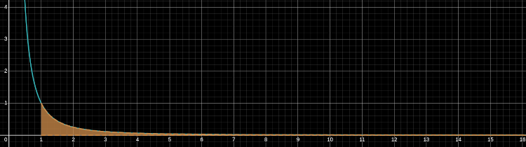
\[\int_1^\infty \frac{1}{x^2}dx \nonumber\]

<p><img src="/assets/math-physics/courses/math2052/rational-x^2-1.png" alt="The area of a curve 1/x^2 from x &gt;= 1" /></p>
<p class="caption">The area under the curve of $\frac{1}{x^2}$ from $x\geq 1$</p>

<p>The remarkable result is that even though the domain is unbounded, the area is finite (equals to 1).</p>

<blockquote>
  <p><strong>Improper Integrals:</strong> Without loss of generality, consider $[a, b)$, where $b$ is finite or $\infty$. Let $f$ be defined on $[a,b)$ and integrable on each $[a,d]$ for $a \lt d \lt b$.</p>

  <p>We define $\int_a^b f(x)dx = \lim\limits_{d\to b^{-}}\int_a^d f(x)dx$, provided the limit exists</p>
</blockquote>

<p>Consider the example: $\int_1^\infty \frac{1}{x^2}dx$:</p>

\[\begin{align*}
\int_1^\infty \frac{1}{x^2}dx &amp;= \lim\limits_{d\to\infty} \int_1^d \frac{1}{x^2}dx \\
&amp;= \lim\limits_{d\to\infty} \left(\frac{x^{-1}}{-1}\bigg|_1^d\right) \\
&amp;= \lim\limits_{d\to\infty} \left( \frac{-1}{d} - \left(-\frac{1}{1}\right) \right) \\
&amp;= \lim\limits_{d\to\infty} \left(1 + \frac{-1}{d}\right) \\
&amp;= 1
\end{align*}\]

<p>Let’s consider the region between $(0, 1]$. Intuitively, since the interval length is only 1 compared to $[1, \infty)$ which has infinite length, surely the area should be finite, right?</p>

<p>Wrong! It turns out that $\int_0^1 \frac{1}{x^2}dx$ diverges (or converges to $\infty$), despite the bounded domain.</p>

<p>As $0\notin dom(f)$, the integral is improper:</p>

\[\begin{align*}
\int_0^1 \frac{1}{x^2} &amp;= \lim\limits_{d\to 0^+} \int_d^1 \frac{1}{x^2}dx \\
&amp;= \lim\limits_{d\to 0^+} \left(\frac{x^{-1}}{-1}\bigg|_d^1\right) \\
&amp;= \lim\limits_{d\to 0^+} \left( \frac{-1}{1} - \left(-\frac{1}{d}\right) \right) \\
&amp;= \lim\limits_{d\to 0^+} \left(\frac{1}{d} - 1\right) \\
&amp;= \infty
\end{align*}\]

<p>We can generalise this behavior by solving $\int_1^\infty \frac{1}{x^p}$ and $\int_0^1 \frac{1}{x^p}$.</p>

\[\begin{align*}
\int_0^1 = \begin{cases} 
      \infty &amp; p \geq 1 \\
      \frac{1}{1-p} &amp; p \lt 1
\end{cases}
\end{align*}\]

<p>and</p>

\[\begin{align*}
\int_1^\infty = \begin{cases}
      \frac{1}{p-1} &amp; p \gt 1 \\
      \infty &amp; p \leq 1
\end{cases}
\end{align*}\]

<blockquote>
  <table>
    <thead>
      <tr>
        <th>Integral</th>
        <th>p &lt; 1</th>
        <th>p = 1</th>
        <th>p &gt; 1</th>
      </tr>
    </thead>
    <tbody>
      <tr>
        <td>$\int_0^1 \frac{1}{x^p} dx$</td>
        <td>Converges</td>
        <td>Diverges</td>
        <td>Diverges</td>
      </tr>
      <tr>
        <td>$\int_1^\infty \frac{1}{x^p}dx$</td>
        <td>Diverges</td>
        <td>Diverges</td>
        <td>Converges</td>
      </tr>
    </tbody>
  </table>
</blockquote>

<p>What we can conclude from the past few examples is that the size of the domain does not matter, but rather its the behaviour of the function within the interval that matters. 
An obvious result but sometimes taken forgranted.</p>

<p>Recall in the previous <a href="../math1052-commentary">course</a>, we explore the $p$-test which stated:</p>

<blockquote>
  <p><strong>P-Series:</strong> $\sum \frac{1}{n^p}$ converges if $p \gt 1$ and diverges if $p\leq 1$</p>
</blockquote>

<p>$\int_1^\infty \frac{1}{x^p}dx$ and $\sum\limits_{n=1}^\infty \frac{1}{n^p}$ both diverge when $p \leq 1$. Is there a pattern between the two? Turns out yes and it’s called the integral test:</p>

<blockquote>
  <p><strong>Integral Test for Infinite Series:</strong> let $N\in\mathbb{Z}$ and suppose $f(x)$ is continuous, decreasing and non-negative on $[N, \infty]$ then $\sum\limits_{n=N}^\infty f(n)$ converges/diverges $\iff$ $\int_N^\infty f(x)dx$ converges/diverges respectively</p>
</blockquote>

<p>It can be difficult to determine whether an infinite series converge or diverge, so the Integral test will be a handy tool.</p>

<p>If an integral is improper at both endpoints, one must split it up into 2 separate improper integrals and evaluate each integral separately.</p>

<blockquote>
  <p><strong>Improper Integrals (Improper at Both Ends):</strong> If $\int_a^b f(x)dx$ is improper at both ends, then by definition $\int_a^b f(x)dx = \int_a^c f(x)dx + \int_c^b f(x) dx$, where $c\in(a,b)$ and $f$ is defined at $c$.</p>

  <p>If one of the two improper integrals evaluates to $\infty$ and the other is $-\infty$, then the integral is undefined</p>
</blockquote>

<p>For instance, consider the following example:</p>

<p><img src="/assets/math-physics/courses/math2052/rational-improper-both-endpoints.png" alt="Area of 1/(1+x^2)" /></p>
<p class="caption">Area of $\frac{1}{1+x^2}$</p>

\[\begin{align*}
\int_{-\infty}^\infty \frac{1}{x^2+1}dx
\end{align*}\]

<p>The two endpoints are improper and thus are broken into two pieces:</p>

<ol>
  <li>$\int_{-\infty}^0 \frac{1}{x^2+1}dx$</li>
  <li>$\int_0^\infty \frac{1}{x^2+1}dx$</li>
</ol>

<p><strong>Important:</strong> Both pieces must converge for the original integral to converge. If even one diverges, the entire integral diverges.</p>

<p>The problem will be left as an exercise to the readers.</p>

<p>A common mistake is to compute an improper integral that is improper at both endpoints as one:</p>

\[\begin{align*}
\int_{-\infty}^\infty x dx &amp;= \lim\limits_{d\to\infty}\int_{-d}^d xdx \\
&amp;= \lim\limits_{d\to\infty} \left(\frac{x^2}{2}\bigg|_{-d}^d\right) \\
&amp;= \lim\limits_{d\to\infty} \frac{d^2}{2} - \left(\frac{(-d)^2}{2}\right) \\
&amp;= 0 \quad\text{ THIS IS WRONG}
\end{align*}\]

<p>By symmetry, this seems fine. But it is <strong>invalid</strong> because the integral is improper at both endpoints and thus must be split. We will soon see that the integral is in fact undefined:</p>

<p>Left Piece:</p>

\[\begin{align*}
\int_{-\infty}^0 x dx &amp;= \lim\limits_{d\to\infty}\int_{-d}^0 xdx \\
&amp;= \lim\limits_{d\to\infty} \frac{x^2}{2}\bigg|_{-d}^0 \\
&amp;= \lim\limits_{d\to\infty} \left(\frac{0^2}{2} - \frac{(-d)^2}{2}\right) \\
&amp;= 0 - \infty \\
&amp;= -\infty
\end{align*}\]

<p>Right Piece:</p>

\[\begin{align*}
\int_{0}^\infty x dx &amp;= \lim\limits_{d\to\infty}\int_{0}^\infty xdx \\
&amp;= \lim\limits_{d\to\infty} \frac{x^2}{2}\bigg|_0^\infty \\
&amp;= \lim\limits_{d\to\infty} \left(\frac{d^2}{2} - \frac{0^2}{2}\right) \\
&amp;= \infty \\
\end{align*}\]

<p>As one diverges to $-\infty$ while the other to $\infty$, we cannot treat the two as equal opposites and thus they do not cancel each other.</p>

<hr />

<p><a name="power"></a></p>
<h2 id="power-series">Power Series</h2>

<p>Have you ever wondered how a calculator computes transcendentals such as $\sin x$ or $e^x$? The secret lies in <strong>power series</strong>, infinite sums of terms 
that represent these functions accurately. Think of a power series as a polynomial with infinitely many terms. For instance, consider 
$e^x$, it can be represented as the following:</p>

\[\begin{align*}
e^x = 1 + x + \frac{x^2}{2} + \frac{x^3}{6} + \frac{x^4}{24} + \cdots = \sum\limits_{n=0}^\infty \frac{x^n}{n!}
\end{align*}\]

<p>Evidentally, calculators must give an answer and thus cannot sum an infinite amount of terms. Therefore, it is important for us to know how many terms 
are enough to sufficiently give us an answer that is precise to our needs. This approximation is a subject that is also explored in this course.</p>

<blockquote>
  <p><strong>Power Series:</strong> let $(a_n)_{n=0}^\infty$ be a sequence. The series $\sum\limits_{n=0}^\infty a_n x^n$ is called a <strong>power series</strong> (centered at 0) with coefficients $(a_n)^\infty_{n=0}$</p>
</blockquote>

<p>In the previous course, we studied series convergence:</p>

\[\sum_{n=0}^{\infty} a_n \nonumber\]

<p>And utilised tests (p-test, ratio test, comparison test, etc.) to answer whether the series converge or diverge. With power series, we face a new question:</p>

\[\sum_{n=0}^{\infty} a_n x^n \nonumber\]

<p>For which values of $x$ does this series converge? The questions and answers we seek is no longer simply whether a series converge but also to determine 
the interval of x-values where converge occurs (called the radius of convergence). In power series, convergence is dependent on $x$, for instance:</p>

\[\begin{align*}
\sum\limits_{n=0}^\infty n^n x^n
\end{align*}\]

<p>By ratio test:</p>

\[\begin{align*}
\lim\limits_{n\to\infty} |n^n x^n|^\frac{1}{n} = \lim_{n \to \infty} n|x| = \begin{cases}
    \infty &amp; x \neq 0 \\
    0 &amp; x = 0
\end{cases}
\end{align*}\]

<p>This power series converges only when $x = 0$. This is consistent to a fact about power series, they always converge when $x = 0$ unsurprisingly.</p>

<blockquote>
  <p><strong>Fact 1:</strong> every power series coverges at $x = 0$ as $0^0 = 1$</p>
</blockquote>

<p>Consider another example: $\sum\limits_{n=0}^\infty x^n$. By geometric series where $x = r$, we have $\sum\limits_{n=0}^\infty x^n = \frac{1}{1-x}$ which converges when $|x| \lt 1$.</p>

<p>Thus, in this example, we have the power series converge when $x \lt 1$, a larger interval compare to the previous example which converged only at one point.</p>

<p>Now consider the last example: $e^x = \sum\limits_{n=0}^\infty \frac{x^n}{n!}$. This is a power series with $a_n = \frac{1}{n!}$. By fixing $x$ and applying the ratio test, we have the following:</p>

\[\begin{align*}
\lim\limits_{n\to\infty} \bigg|\frac{\frac{1}{(n+1)!} x^{n+1}}{\frac{1}{n!} x^n}\bigg| &amp;=  \lim\limits_{n\to\infty} \bigg| \bcancel{\left(\frac{n!x^n}{n!x^n}\right)} \frac{x}{(n+1)}\bigg|\\
&amp;= \lim\limits_{n\to\infty} \frac{|x|}{n+1} \\
&amp;= |x| \lim\limits_{n\to\infty} \frac{1}{n+1} \\
&amp;= 0 \lt 1
\end{align*}\]

<p>So by ratio test, $\sum\limits_{n=0}^\infty \frac{x^n}{n!}$ converges and since $x$ was arbitrary, it converges $\forall x\in\mathbb{R}$</p>

<p>The last 3 examples illustrates 3 possibilities for a power series $\sum a_nx^n$, it can either:</p>
<ol>
  <li>converge only at $x = 0 \implies R = 0$</li>
  <li>converges for all $x$ in a bounded interval certered at 0</li>
  <li>converges $\forall x\in\mathbb{R} \implies R = \infty$</li>
</ol>

<blockquote>
  <p><strong>Theorem 7 (Radius of Convergence):</strong> For the power series $\sum\limits_{n=0}^\infty a_n x^n$, let $R = \lim\limits_{n\to\infty} \bigg| \frac{a_n}{a_{n+1}} \bigg|$</p>

  <p>Then $\sum\limits_{n=0}^\infty a_n x^n$ converges absoutely for $|x| \lt R$ and diverges for $|x| \gt R$</p>

  <p>where $R$ is called the <strong>radius of convergence</strong> of $\sum\limits_{n=0}^\infty a_n x^n$</p>
</blockquote>

<p><strong>Note:</strong> Endpoints to be checked separately</p>

<p><strong>Example:</strong> Find radius of convergence of $\sum\limits_{n=1}^\infty \frac{x^n}{n}$</p>

<p>$\sum\limits_{n=1}^\infty \frac{x^n}{n} = \sum\limits_{n=1}^\infty a_nx^n$, where $a_n=\frac{1}{n}$</p>

\[\lim\limits_{n\to\infty} \bigg|\frac{a_n}{a_{n+1}}\bigg| = \lim\limits_{n\to\infty} \bigg|\frac{\frac{1}{n}}{\frac{1}{n+1}}\bigg| = \lim\limits_{n\to\infty} \bigg|\frac{n+1}{n}\bigg| = 1 \nonumber\]

<p>Since this limit exists, $R = 1$. Hence, $\sum\limits_{n=1}^\infty \frac{x^n}{n}$ converges $\forall x$ with $|x| \lt 1$ i.e. $\forall x\in(-1,1)$</p>

<p>We need to check the endpoints separately since it may converge over there as well.</p>

<p>For $x = -1$:</p>

\[\sum\limits_{n=1}^\infty \frac{x^n}{n} = \sum\limits_{n=1}^\infty \frac{(-1)^n}{n}\nonumber\]

<p>This converges by the alternating series test.</p>

<p>For $x = 1$:</p>

\[\sum\limits_{n=1}^\infty \frac{x^n}{n} = \sum\limits_{n=1}^\infty \frac{1^n}{n}\nonumber\]

<p>Recall this is a harmonic series and thus diverges</p>

<p>Thus, $\sum\limits_{n=1}^\infty \frac{x^n}{n}$ converges for $x\in[1, 1)$.</p>

<p>Note that the radius of convergence is still 1, but we call $[-1,1)$ the <strong>interval of convergence</strong> which could be larger than your radius of convergence itself.</p>

<blockquote>
  <p><strong>Center of Power Series:</strong> Power series can be centered at values other than 0. For a power series centered at $x = x_o$, it is represented as $\sum\limits_{n=0}^\infty a_n(x-x_o)^n$</p>

  <p>The power series converges on $|x-x_o|\lt R$ and diverges on $|x-x_o| \gt R$. Again, the endpoints needs to be checked separately.</p>
</blockquote>

<p><strong>Example:</strong> Find the interval of convergence of $\sum\limits_{n=0}^\infty \frac{5^n}{n}(x-2)^n$</p>

<ol>
  <li>
    <p>Find the radius of convergence:
 $a_n = \frac{5^n}{n}$ so:</p>

\[\begin{align*}
 \lim\limits_{n\to\infty} \bigg|\frac{a_n}{a_{n+1}}\bigg| &amp;= \lim\limits_{n\to\infty}\bigg|\frac{\frac{5^n}{n}}{\frac{5^{n+1}}{n+1}} \\
 &amp;= \lim\limits_{n\to\infty} \left( \frac{5^n}{n} \right)\left(\frac{n+1}{5^{n+1}}\right) \\
 &amp;= \frac{1}{5}\lim\limits_{n\to\infty} \frac{n+1}{n} \\
 &amp;= \frac{1}{5}
 \end{align*}\]

    <p>Thus $\boxed{R = \frac{1}{5}}$ and $x\in(x_o - R, x_o + R) = (2 - \frac{1}{5}, 2 + \frac{1}{5}) = (\frac{9}{5}, \frac{11}{5})$</p>
  </li>
  <li>
    <p>Check endpoints:
 For $x = \frac{9}{5}$:</p>

\[\begin{align*}
 \sum\limits_{n=1}^\infty\frac{5^n}{n}\left(\frac{9}{5} - 2\right)^n &amp;= \sum\limits_{n=1}^\infty\frac{5^n}{n}\left(\frac{-1}{5}\right)^n \\
 &amp;= \sum\limits_{n=1}^\infty\frac{5^n}{n}\left(\frac{(-1)^n}{5^n}\right) \\
 &amp;= \sum\limits_{n=1}^\infty\frac{\bcancel{5^n}}{n}\left(\frac{(-1)^n}{\bcancel{5^n}}\right) \\
 &amp;= \sum\limits_{n=1}^\infty \frac{(-1)^n)}{n}
 \end{align*}\]

    <p>By the alternating test, the series converges</p>

    <p>For $x = \frac{11}{5}$:</p>

\[\begin{align*}
 \sum\limits_{n=1}^\infty\frac{5^n}{n}\left(\frac{11}{5} - 2\right)^n &amp;= \sum\limits_{n=1}^\infty\frac{5^n}{n}\left(\frac{1}{5} - 2\right)^n \\
 &amp;= \sum\limits_{n=1}^\infty \frac{1}{n}
 \end{align*}\]

    <p>As this is a harmonic series, the series converges at $x= \frac{11}{5}$</p>
  </li>
</ol>

<p>Therefore, the interval of convergence for this power series centered at $x_o = 2$ is $[\frac{9}{5}, \frac{11}{5})$</p>

<p>As power series are a function of $x$ on its interval of convergence, a natural question in calculus is:</p>
<ul>
  <li>is it continuous</li>
  <li>is it differentiable</li>
  <li>is it integrable</li>
</ul>

<p>Power series is an accumulation over a sequence of functions, more specifically an accumulation of polynomials which we know are continuous. However, just because each function in a sequence is continuous 
and converges to some function $f$, it does not mean the convergent function $f$ is continuous itself. Therefore, to guard this continuity property in convergent functions, we will need a different notion 
or type of convergence, the uniform convergence. First we shall describe a type of convergence that does not guarantee continuity to the convergent function:</p>

<blockquote>
  <p><strong>Pointwise Convergence:</strong> Let $(f_n)$ be a sequence of funtions. We say that $(f_n)$ <strong>CONVERGES POINTWISE</strong> to $f$ on a set $S$ if $\forall x\in S$, the sequence $f_n(x)$ converges to $f(x)$</p>

  <p><strong>Note:</strong> Does not guarantee $f$ is continuous even if each $f_n$ is continuous</p>
</blockquote>

<p>That is to say:</p>

<blockquote>
  <p><strong>Pointwise Convergence:</strong> $f_n\to f$ pointwise on $S$ if $\forall x\in S, \lim\limits_{n\to\infty} f_n(x)=f(x)$</p>

  <p>i.e. $\forall x\in S, \forall \epsilon \gt 0 \exists N $ such that $n \gt N \implies |f_n(x)-f(x)|\lt \epsilon$</p>
</blockquote>

<p>A counterexample to the preservation of continuity to the convergent function  presented in the textbook is the following sequence $f_n(x) = x^n$ on $[0,1]$. $f_n \to f$ pointwise on [0,1] but is not continuous as:</p>

\[f(x) = \begin{cases}
    0 &amp; x\in[0,1) \nonumber\\
    1 &amp; x = 1
\end{cases}\]

<p>Similarly to how uniform continuity differs from regular continuity by choosing a $\delta$ not dependent on $x$, uniform convergence also tries to pick a $N$ such that it only depends on $\epsilon$ and not $x$. 
The idea is to have the values $f_n(x)$ be ``uniformly” close to the values of $f(x)$ for all $x$:</p>

<blockquote>
  <p><strong>Uniform Convergence:</strong> The sequence of function $(f_n)$ on $S\subseteq \mathbb{R}$ <strong>CONVERGES UNIFORMLY</strong> to a function $f$ on $S$ if $\forall \epsilon \gt 0, \exists N $ such that $n \gt N\implies |f_n(x) - f(x)|\lt \epsilon \forall x\in S$</p>
</blockquote>

<p>Uniform convergence is a stronger type of convergence as it applies to all $x$ and thus we have the following relation:</p>

<blockquote>
  <p>$(f_n)$ converges to $f$ uniformly $\implies (f_n)$ converges to $f$ pointwise</p>
</blockquote>

<p>This should not come to no surprise since if $(f_n)$ converges uniformly, it should converge to $f$ in a subset of $\mathbb{R}$.</p>

<p>The contraire does not hold unexpectedly:</p>

<blockquote>
  <p>$(f_n)$ converges to $f$ pointwise $\bcancel{\implies} (f_n)$ converges to $f$ uniformly</p>
</blockquote>

<p><strong>Example:</strong> $f_n(x) = x^n$ on $[0,1]$. Recall that $f_n$ converges pointwise to:</p>

\[f(x) = \begin{cases}
    0 &amp; x\in[0,1) \nonumber\\
    1 &amp; x = 1
\end{cases}\]

<p>But does it converge uniformly as well? Spoiler it does not, the reason we motivated uniform convergence is to show the preservation of continuity which will come next.</p>

<p>Suppose by contraction that it does.</p>

<p>Then take $\epsilon = \frac{1}{2}$, I can find $N$ such that</p>

<p>$n \gt N \implies |f_n(x) - f(x)| \lt \frac{1}{2} \forall x \in [0,1]$.</p>

<p>In particular, for $n = N+ 1 \gt N$ and $\forall x\in [0,1)$, we have:</p>

<p>$f(x) = 0 \implies |f_{N+1}(x) - f(x)| = |f_{N+1}(x)| = x^{N+1} \lt \frac{1}{2} \forall x\in [0,1)$.</p>

<p>Rearranging,</p>

\[x^{N+1} \lt \frac{1}{2} \implies x \lt \frac{1}{2^\frac{1}{N+1}} \forall x\in [0,1) \quad (*) \nonumber\\\]

<p>From here, I can think of two approaches:</p>

<ol>
  <li>
    <p><strong>Limit Argument:</strong> Since $x^{N+1}$ is continuous and $x^{N+1} \lt \frac{1}{2} \forall x\in [0,1)$:</p>

    <p>We have $1 = \lim\limits_{x\to 1^-} x^{N+1} \lt \frac{1}{2}$ which is a contradiction.</p>
  </li>
  <li>
    <p><strong>Explicit Construction:</strong> We begin with the obvious fact that $1 \lt 2$ and build up to get $1 \lt 2^\frac{1}{N+1}$ and then choose an $L$ such that a contradiction arrives:
 \(\begin{align*}
 2 \gt 1 &amp;\implies 2^\frac{1}{N+1} \gt 1^\frac{1}{N+1} \\
 &amp;\implies 2^\frac{1}{N+1} \gt 1
 \end{align*}\)</p>

    <p>By the density of $\mathbb{Q}, \exists L\in\mathbb{Q}\subset \mathbb{R}$ such that $\frac{1}{2^\frac{1}{N+1}} \lt L \lt 1$.</p>

    <p>By choosing such an $L$ that meets this criteria, we have $L\in[0,1)$ such that $L \gt \frac{1}{2^\frac{1}{N+1}}$ but by (*) we also have $L \lt \frac{1}{2^\frac{1}{N+1}}$ which is a contradiction.</p>
  </li>
</ol>

<p>Let us now show an example in how to prove something is uniform convergent:</p>

<p><strong>Example:</strong> Let $f_n(x) = \frac{1}{n}\sin(nx)$ for $x\in\mathbb{R}$. Prove that $f_n\to 0$ uniformly.</p>

<p>Rough Work: Let $\epsilon \gt 0$ be given. Then,</p>

\[\begin{align*}
|f_n(x) - f(x)| &amp;= |\frac{1}{n}\sin(nx) - 0| \\
&amp;= \frac{1}{n}|\sin(nx)|\leq \frac{1}{n} \forall x \\
\frac{1}{n} &amp;\underset{\text{ want}}{&lt;} \epsilon \implies n \gt \frac{1}{\epsilon}
\end{align*}\]

<p>Choose $N = \frac{1}{\epsilon}$.</p>

<blockquote>
  <p><strong>Heurestic to show Uniform Convergence:</strong> In your rough work, you want to bound the function such that it is not dependent on $x$ such as $\frac{1}{n}$</p>

  <p>e.g. take $N = \frac{1}{\epsilon}$ for instance where it does not depend on $x$ in a uniform convergence proof</p>
</blockquote>

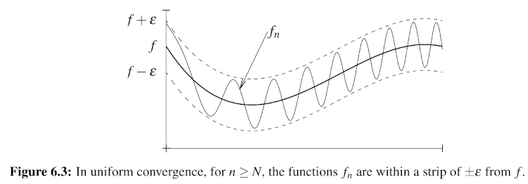
<p><img src="/assets/math-physics/courses/math2052/uniform-convergence.png" alt="A diagram trying to illustrate uniform convergence" /></p>
<p class="caption">An illustration how $f_n$ is bounded to the $\epsilon$ window and as $\epsilon$ gets smaller, the $f_n$ gets squeezed but remains in the window. i.e. Eventually as you go further down the sequence (a larger $N$), you will eventually find a function flat enough to squeeze into the window. Extracted from <a href="https://ocw.mit.edu/courses/18-100a-real-analysis-fall-2020/mit18_100af20_basic_analysis.pdf">MIT OCW Real Analysis Notes</a></p>

<p>Now we have seen what it means for a function to converge pointwise and uniformly, let us now revisit the purpose of introducing a strongegr notion of convergence (uniform convergence):</p>

<blockquote>
  <p>$f_n$ is continuous $\forall n$ and $f_n \to f$ pointwise $\bcancel{\implies} f$ is continuous</p>
</blockquote>

<p>But</p>

<blockquote>
  <p>$f_n$ is continuous $\forall n$ and $f_\to f$ uniformly $\implies f $ is continuous</p>
</blockquote>

<blockquote>
  <p><strong>Theorem (Uniform Convergence Preserving Continuity):</strong> let $(f_n)$ be a sequence of functions on $S$ such that $f_n \to f$ converges uniformly.
If each $f_n$ is continuous, so is $f$</p>
</blockquote>

<p>If we take the contrapositive of this theorem above, we obtain another tool to disprove uniform convergence:</p>

<blockquote>
  <p><strong>Disproving Uniform Convergence via Continuity:</strong> If $f_n \to f$ pointwise and each $f_n$ is continuous but $f(x)$ is not continuous, then this convergence is not uniform</p>
</blockquote>

<p>Before proceeding to the consequences of uniform convergence and the preservation of continuity, let’s revisit our favorite function in this chapter: $f_n(x) = x^n$ and recall 
that $f_n \to f$ pointwise on $[0,1]$ where,</p>

\[f(x) = \begin{cases}
    0 &amp; x\in[0,1) \nonumber\\
    1 &amp; x = 1
\end{cases}\]

<p>This does not uniformly converge to $f$ as it was discontinuous at $x = 1$. But what about for $x\in[0,1)$?</p>

<p>For $f_n = x^n$ on $[0,1), \lim\limits_{n\to\infty} f_n(x) = 0 \forall x$</p>

<p>The constant function $0$ is continuous $\forall x$ but is it uniformly convergent on $[0,1)$? NO, we showed previously that it did not</p>

<p>What about from a fixed positive number $b \lt 1$. We will make the claim that on $[0,b], f_n \to 0$ uniformly:</p>

<p>Rough Work: Let $\epsilon \gt 0$. We want $N$ such that $n \gt N$:</p>

\[\begin{align*}
|x^n - 0| \lt \epsilon \forall x\in [0,b] \\
|x^n| = x^n \leq b^n \underset{\text{want}}{\lt} \epsilon
\end{align*}\]

<p><strong>Note:</strong> $b^n \lt \epsilon$ is only possible because $b \lt 1$ thus $b^n \lt 1$ (i.e. for $b\lt 1 \implies b^{N+1} \lt b^{N}$)</p>

<p>Thus we have,</p>

\[\begin{align*}
b^n \lt \epsilon &amp;\iff n\ln b \lt \ln \epsilon \\
&amp;\iff n \gt \frac{\ln\epsilon}{\ln b}, \quad \text{inequality flipped because if $b\lt 1$ then $\ln b \lt 0$}
\end{align*}\]

<p>Thus choose $N = \frac{\ln\epsilon}{\ln b}$</p>

<p>In conclusion, for the examples, we have seen for $f_n(x) = x^n$,</p>

<p>\(f(x) = \begin{cases} 
    0 &amp; 0\leq x \lt 1 \\ 
    1 &amp; x = 1
\end{cases}\)</p>
<ul>
  <li>on $[0,1], f_n \to f$ pointwise but not uniformly</li>
  <li>on $[0,1), f_n \to 0$ pointwise but not uniformly</li>
  <li>on $[0,b]$ for $b \lt 1, f_n \to 0$ uniformly</li>
</ul>

<p>I recall being a bit surprised by this result how fixing a point allows $f_n$ converge uniformly to $f$. But now that I think of it, if we were to start plugging in numbers as $x \to 1$, we’ll notice the 
following:</p>

<ul>
  <li>$x = 0.5: 0.5^n \to 0$ fast ($N_1 &gt; N$)</li>
  <li>$x = 0.9: 0.9^n \to 0$ slowly (i.e. $N_2 » N_1 &gt; N$)</li>
  <li>$x = 0.99: 0.99^n \to 0$ even slower (i.e. $N_3 »&gt; N_2 » N_1 &gt; N$)</li>
  <li>$x \to 1: x^n \to 0$ extremely and arbitrarily slowly  (i.e. $N_4 »»»»»»» N_3 »&gt; N_2 » N_1 &gt; N$)</li>
</ul>

<p>Thus as $x\to 1$, we observe the growth to converge $f_n(x)$ to 0 get slower and slower</p>

<p>We can now say the following:</p>

<blockquote>
  <p><strong>Theorem:</strong> let $(t_n)$ be a sequence of continuous function on $[a,b]$ which converges uniformly to $f$.</p>

  <p>Then $\lim\limits_{n\to\infty} \int_a^b f_n(x)dx = \int_a^b \lim\limits_{n\to\infty} f_n(x)dx = \int_a^b f(x)dx$</p>
</blockquote>

<p>Previously, we saw that $f_n = x^n$ does not converge uniformly from [0,1) as the terms converges to $f$ so slowly. In <a href="../math1052-commentary">MATH1052</a>, we introduced cauchy sequences, a sequence that 
converges and exhibits a behavior whereby after some $N$, the distance of any two functions in the sequence are arbitrarily so close that convergence is guaranteed.</p>

<blockquote>
  <p><strong>Cauchy Sequences:</strong> a sequence $(s_n)$ is cauchy if $\forall \epsilon \gt 0, \exists N $ such that $m,n \gt N \implies |a_n-a_m| \lt \epsilon$</p>
</blockquote>

<blockquote>
  <p>$(s_n)$ is cauchy $\iff (s_n)$ is convergent</p>
</blockquote>

<p>We want a similar result for functions because if you recalled, this entire section is dedicated to power series which are infinite series of functions (even though it may not seem like it with our 
discussion in sequences and convergence).</p>

<blockquote>
  <p><strong>Uniformly Cauchy:</strong> a sequence $(f_n)$ of functions on $S\subseteq \mathbb{R}$ is called <strong>UNIFORMLY CAUCHY</strong> if $\forall \epsilon \gt 0, \exists N$ such that $m,n \gt N \implies |f_n(x) - f_m(x)| \lt \epsilon \quad\forall x\in S$</p>
</blockquote>

<p>To tie this together with uniform convergent, we have the following result:</p>

<blockquote>
  <p><strong>Lemma:</strong> if $f_n \to f$ uniformly then it is uniformly cauchy</p>
</blockquote>

<p>and</p>

<blockquote>
  <p><strong>Theorem:</strong> Let $(f_n)$ be a uniformly cauchy sequence of functions on $S\subseteq \mathbb{R}$ then $\exists$ a function $f$ on $S$ such that $f_n\to f$ uniformly</p>
</blockquote>

<p>Thus far, we have talked about functions in a sequence but never tied it with power series. Let us now be equipped with what it means for a series of functions to a power series:</p>

<blockquote>
  <p>$\sum\limits_{k = 0}^\infty g_k(x)$ is a power series of functions if $g_k(x) = a_kx^k$</p>
</blockquote>

<p>For instance, the following function is a series of function but is not a power series of functions: $\sum\limits_{k=0}^\infty \frac{x^k}{1+x^k}$ because it is not in the right form.</p>

<blockquote>
  <p><strong>Uniform Convergence of Function Power Series:</strong> let $\sum\limits_{k=0}^\infty g_k(x)$ be a series of functions on $S$ such that each $g_k$ is continuous.
If $\sum\limits_{k=0}^\infty g_k(x)$ is uniformly convergent to $g(x)$, then $g$ is continuous</p>
</blockquote>

<p>This result should not be of any surprise as we previously saw that</p>
<ul>
  <li>sums of continuous functions are continuous</li>
  <li>uniform convergence preserves continuity among convergent sequences of functions</li>
</ul>

<p>Let us now introduce another equivalence relation to uniformly cauchy in respect to function power series:</p>

<blockquote>
  <p><strong>Uniform Cauchy Definition for $\sum\limits_{k=0}^\infty g_k(x)$:</strong> $\sum\limits_{k=0}^\infty g_k(x)$ is uniformly cauchy on $S$</p>

  <p>$\iff \forall \epsilon \gt 0, \exists N $ such that $m,n \gt N \implies |\sum\limits_{k=0}^n g_k(x) - \sum\limits_{k=0}^m g_k(x)|\lt \epsilon$</p>

  <p>$\iff \forall \epsilon \gt 0, \exists N $ such that $n\geq m \gt N \implies |\sum\limits_{k=m}^n g_k(x)| \lt \epsilon$</p>
</blockquote>

<p>Now that we have seen what it means for a power series to uniformly converge, we can now introduce a nice test to determine whether it converges uniformly:</p>

<blockquote>
  <p><strong>Weierstrass M-Test:</strong> let $(M_K)$ be a sequence of non-negative numbers with $\sum\limits_{k=0}^\infty M_k \lt \infty$.
If $|g_k(x)| \leq M_k \forall x\in S$, then $\sum\limits_{k=0}^\infty g_k(x)$ converges uniformly on $S$</p>
</blockquote>

<p>Let us see an example of how to utilise this test to determine whether an infinite function power series converges ot a continuous function:</p>

<p><strong>Example:</strong> Show that $\sum\limits_{k=0}^\infty \frac{1}{n^2}\sin(nx)$ converges to a continuous function on $\mathbb{R}$</p>

<p>First note that: $|\frac{1}{n^2}\sin(nx)| = \frac{1}{n^2}|\sin(nx)|\leq \frac{1}{n^2}$</p>

<p>Let $M_n = \frac{1}{n^2}$. Then $\sum\limits_{k=0}^\infty M_n = \sum\limits_{k=0}^\infty \frac{1}{n^2} \lt \infty$ by P-series</p>

<p>So by M-test, $\sum\limits_{k=0}^\infty \frac{1}{n^2}\sin(nx)$ converges uniformly on $\mathbb{R}$
Since $g_n(x) = \frac{1}{n^2}\sin(nx)$ is continuous on $\mathbb{R} \forall n$ and converges uniformly, the limit must be continuous.</p>

<blockquote>
  <p><strong>Recall:</strong> if $\sum\limits_{k=0}^\infty a_k$ is a series of numbers then $\sum\limits_{k=0}^\infty a_k$ converges $\implies \lim\limits_{n\to\infty} a_n = 0$</p>

  <p>Though the opposite direction does not hold (think of $\sum \frac{1}{n}$ diverges by P-series but the limit is 0.
We have an analogous version of this fact for series of functions:</p>
</blockquote>

<blockquote>
  <p>if $\sum\limits_{k=0}^\infty g_k(x)$ converges uniformly on $S$ then $\lim\limits_{n\to\infty} \sup\{|g_n(x)| : x\in S\} = 0$</p>
</blockquote>

<p>One consequence of this lemma above is that we can use the contrapositive to conclude whether a function power series does not converge uniformly, which is probably a much more useful fact:</p>

<blockquote>
  <p>if one can show $\lim\limits_{n\to\infty} \sup\{|g_n(x)| : x\in S\} \neq 0$, then one can conclude that $\sum g_k(x)$ does not converge uniformly on $S$</p>
</blockquote>

<p><strong>Example:</strong> Consider the power series $\sum \frac{x^n}{3^n}$</p>

<p>Before utilising our new tool to determine whether this power series converges uniformly, let’s establish the convergence interval:</p>

<p>Note that the radius of convergence is 3: $R = \lim\limits_{n\to\infty}\left|\frac{a_n}{a_{n+1}}\right| = \left|\frac{\frac{1}{3^n}}{\frac{1}{3^{n+1}}}\right| = 3$</p>

<p>At $x = 3: \sum 1 = \infty$ and at $x = -3: \sum(-1)^n$ diverges. Thus our interval of convergence is: $I = (-3,3)$</p>

<p>Using the new tool, we have $\sup\{|\frac{x^n}{3^n}| : x\in (-3,3)\} = 1 \forall n$ so $\lim_{x\to\infty} \sup\{|\frac{x^n}{3^n}| : x\in (-3,3)\} = 1 \neq 0$</p>

<p>So by the lemma, we know $\sum \frac{x^n}{3^n}$ does not converge uniformly on $(-3,3)$</p>

<p>But what if we restricted the interval to a concrete number similar to how we found $f_n(x) = x^n$ converges uniformly if we restricted $S$ from $[0,1)$ to $[0, b]$. It turns out if we restrict 
the endpoints of our interval of convergence to be smaller and concrete, our once non-uniformly convergent sequence/power series does converge.</p>

<blockquote>
  <p><strong>Theorem:</strong> let $\sum a_n x^n$ be a power series with a radius of convergence $R \gt 0$. If $0 \lt b \lt R$, then the power series converges uniformly on $[-b,b]$ and converges to a continuous function on 
$(-R,R)$</p>
</blockquote>

<p>Let’s revisit the previous example and restrict the interval to $b \lt R = 3$. For this exercise, we will avoid invoking the theorem above and show you the lengthy process to obtain the same result:</p>

<p>Let $b\in(0,3)$ so if $x = b\implies \sum \frac{b^n}{3^n} = \sum\left(\frac{b}{3}\right)^n$ converges by gemoetric series (as $0 \lt b \lt 3$)</p>

<ol>
  <li>
    <p>To show $\sum \frac{x^n}{3^n}$ converges uniformly on $[-b,b]$, we can utilise the Weierstrass M-test: $\forall x\in [-b,b], \left|\frac{x^n}{3^n} \right | \leq \left|\frac{b^n}{3^n}\right| = \left(\frac{b}{3}\right)^n = M_n$.
 Since $\sum M_n$ converges, by the Weierstrass M-test, $\sum\frac{x^n}{3^n}$ converges uniformly on $[-b,b]$.</p>
  </li>
  <li>
    <p>Now all that is left is to show $\sum \frac{x^n}{3^n}$ converges to a continuous function on $[-b,b]$:</p>

    <p>Note that $\frac{x^n}{3^n}$ is continuous on $\forall n$. Thus, $\sum\frac{x^n}{3^n}$ is continuous on $[-b,b] \forall b\in[0,3)$. As $b$ is arbitrary, $\sum \frac{x^n}{3^n}$ converges to a continuous function on $(-3, 3)$.</p>
  </li>
</ol>

<p>This is definitely much longer than simply invoking the theorem which gives us both uniformly convergence and convergence to a continuous function for free: Since $R = 3 \gt 0$ and $b \in (0,R)$, by the theorem above, we have $\sum \frac{x^n}{3^n}$ converges uniformly on $[-b,b]$ and converges to a continuous function on $(-3,3)$.</p>

<p>Recall that one of the motivations of utilising power series is to represent transcendental functions such as $e^x$ as an infinite series of polynomials. What would be desirable is if we 
could differentiate and integrate power series term by term. For instance, it would be nice if we could do the following</p>

\[\begin{align*}
\left(\sum\limits_{n=0}^\infty a_nx^n\right)' &amp;= (a_0 + a_1x + a_2x^2+\cdots)' \overset{?}{=} a_1 + 2a_2x+3a_3x^2+\cdots \overset{?}{=} \sum\limits_{n=1}^\infty na_nx^{n-1} \\
\int \sum\limits_{n=0}^\infty a_nx^ndx &amp;\overset{?}{=} \sum\limits_{n=0}^\infty \frac{a_nx^{n+1}}{n+1}
\end{align*}\]

<p>But for these properties to work, we must ensure that the radius of convergence remains the same in these new forms:</p>

<blockquote>
  <p><strong>Lemma:</strong> If $\sum\limits_{n=0}^\infty a_n x^n$ has a radius of convergence $R$, then so does $\sum\limits_{n=1}^\infty na_nx^{n-1}$ and $\sum\limits_{n=0}^\infty \frac{a_n}{n+1}x^{n+1}$</p>
</blockquote>

<p>As the radius of convergence remains the same even after taking the form of what seems like to be its differentiatiable and integrable equivalences, let us now introduce the theorem that 
ties this together to permit us to integrate and differentiate the series term by term:</p>

<blockquote>
  <p><strong>Theorem:</strong> Suppose $f(x) = \sum_{n=0}^\infty a_nx^n$ has a radius of convergence $R \gt 0$. Then,
$\int_0^x f(t)dt = \sum\limits_{n=0}^\infty \frac{a_n}{n+1}x^{n+1}$ for $|x| \lt R$</p>
</blockquote>

<blockquote>
  <p><strong>Theorem:</strong> Let $f(x) = \sum_{n=1}^\infty a_nx^n$ have radius of convergence $R \gt 0$. Then $f$ is differentiable on $(-R,R)$ and</p>

  <p>$f’(x) = \sum_\limits{n=1}^\infty na_nx^{n-1}$ for $|x| \lt R$</p>

  <p><strong>Note:</strong> Notice that the index changes from 0 to 1 in the differentiable form. The index does not change for the integral</p>
</blockquote>

<p>Thus far. the previous theorem only discusses differentiablity at the open intervals $(-R, R)$ but what about at its endpoint? That is what the next theorem, Abel’s Theorem, attempts to tackle. 
We know from last year that differentiability implies continuity (i.e. to be differentiable at $x = a$, then by definition, it must also be continuous at $a$)</p>

<blockquote>
  <p><strong>Abel’s Theorem:</strong> let $f(x) = \sum a_nx^n$ have a radius of convergence $R \gt 0$, $R \lt \infty$. If $\sum a_nx^n$ converges at $x = R$, then it is continuous there. The same is true at $x = -R$.</p>
</blockquote>

<p>As a consequence, we have that every power series converge to a continuous function on its entire interval of convergence including at its endpoint provided it is defined and does indeed converge there.</p>

<blockquote>
  <p>Every power series converges to a continuous function on its entire interval of convergence (including its endpoints if defined and converges there)</p>

  <p>i.e. $\sum \frac{x^n}{n^2}$ has an interval of convergence (I.O.C) on $[-1,1]$ and thus is continuous on $[-1,1]$</p>
</blockquote>

<hr />

<p><a name="taylor"></a></p>
<h2 id="taylor-series">Taylor Series</h2>

<p>Recall that one of the motivations of power series is to represent transcendental functions as an infinite series of polynomials. This is the math that allows calculators be able to compute $e^x$ for 
instance within an acceptable error or to allow oneself to integrate a complicated expression into simple series of polynomials. However, how does one translate a function such as $e^x$ or $\sin(x)$ 
into a series of polynomials? That is what will be explored in this section, working with taylor series which gives us a methodical way to transform a function into a power series.</p>

<blockquote>
  <p><strong>Taylor Series:</strong> let $f$ be defined on an open interval containing $x_o$. Suppose that all order of derivatives of $f$ exist at $x_o$.
Then the series</p>

  <p>$\sum\limits_{n=0}^\infty \frac{f^{(n)}(x_o)}{n!}\left(x-x_o\right)^n$ is called the taylor series for $f$ about $x_o$</p>

  <p>For $n\geq 1$, the remainder $R_n(x)$ is defined by:</p>

  <p>$R_n(x) = f(x) - \sum\limits_{k=0}^{n-1}\frac{f^{(k)}(x_o)}{k!}(x-x_o)^k$</p>
</blockquote>

<p>When we approximate a function $f(x)$ using a finite Taylor polynomial of degree $n$ which we call $P_n(x)$, the approximation is rarely perfect. This difference must be taken into account and thus the remainder</p>

\[\begin{align*}
R_n(x) &amp;= f(x) - \sum\limits_{k=0}^{n-1} \frac{f^{(k)}(c)}{k!}(x-c)^k \\
f(x) &amp;= \sum\limits_{k=0}^{n-1} \frac{f^{(k)}(c)}{k!}(x-c)^k + R_n(x) \\
f(x) &amp;= P_n(x) + R_n(x)
\end{align*}\]

<p>On a note about the remainder, we also have this result:</p>

<blockquote>
  <p>$f(x) = \sum\limits_{k=0}^\infty \frac{f^{(k)}(x_o)}{k!}(x-x_o)^k \iff \lim\limits_{n\to\infty}R_n(x) = 0$</p>
</blockquote>

<p>Suppose we have a power series in the form $f(x) = \sum a_n(x-x_o)^n$. We have never discussed how to determine what $a_n$ is. In our definition of taylor series, all order of derivatives of $f$ exists at $x_o$. 
This,</p>

\[\begin{align*}
f(x) &amp;= a_o + a_1(x-x_o) + a_2(x-x_o)^2 + a_3(x-x_o)^3 + \cdots \\
f'(x) &amp;= a_1 + 2a_2(x-x_o) + 3a_3(x-x_o)^2 + \cdots \\
f''(x) &amp;= 2a_2 + (3)(2)a_3(x-x_o) + 4(3)a_4(x-x_o)^2 + \cdots \\
f'''(x) &amp;= 3(2)a_3 + 4(3)(2)a_4(x-x_o) + 5(4)(3)a_5(x-x_o)^2 + \cdots
\end{align*}\]

<p>Let $x = x_o$, then:</p>

\[\begin{align*}
f(x_o) &amp;= a_o &amp;= 0!a_o \\
f'(x_o) &amp;= a_1 &amp;= 1! a_1 \\
f''(x_o) &amp;= 2a_2 &amp;= 2!a_2 \\
f'''(x_o) &amp;= 3(2)a_3 &amp;= 3! a_3
\end{align*}\]

<p>Then by induction, we have:</p>

\[\begin{align*}
f^{(n)} = n!a_n\\
\boxed{a_n = \frac{f^{(n)}(x_o)}{n!}}
\end{align*}\]

<blockquote>
  <p><strong>Taylor Coefficient:</strong> $a_n = \frac{f^{(n)}(x_o)}{n!}$</p>
</blockquote>

<p>Let us now go through an example to determine the taylor series of $\sin(x)$ centered at 0 (Note: This is also called a Maclaurin Series, a Taylor series centered at 0).</p>

<p>First let’s observe the orders of the derivatives of $\sin(x)$:</p>

\[\begin{align*}
f(x) &amp;= \sin(x)  &amp; f(0) &amp;= 0 \\
f'(x) &amp;= \cos(x) &amp; f'(0) &amp;= 1 \\
f''(x) &amp;= -\sin(x) &amp; f''(0) &amp;= 0 \\
f^{(3)}(x) &amp;= -\cos(x) &amp; f^{(3)}(0) &amp;= -1 \\
f^{(4)}(x) &amp;= \sin(x) &amp; f^{(4)}(0) &amp;= 0 \\
\cdots
\end{align*}\]

<p>So we have: 
\(f^{(n)}(0) = \begin{cases}
0 &amp; \text{if n is even} \\
1 &amp; \text{if n = 4k+1} \\
-1 &amp; \text{if n = 4k+3}
\end{cases}\)</p>

<p>and $a_n = \frac{f^{(n)}(0)}{n!}$ so the taylor series of $\sin(x)$ around 0 is</p>

\[\begin{align*}
\sum\limits_{k=0}^\infty \frac{f^{(k)}(0)}{k!}x^k &amp;= x - \frac{x^3}{3!} + \frac{x^5}{5!} - \frac{x^7}{7!} + \cdots \\
&amp;= \sum\limits_{n=0}^\infty \frac{(-1)^nx^{2n+1}}{(2n+1)!}
\end{align*}\]

<p>Let’s now explore the one applications of taylor series I hinted at in the beginning to better understand the power of formulating a function as a taylor series:</p>

<p><strong>For Approximations:</strong></p>

<p>How many terms do we need to approximate $\sqrt{e} = e^\frac{1}{2} = \sum\limits_{n=0}^\infty \frac{\left(\frac{1}{2}\right)^n}{n!}$ with an error less than $0.0001$?</p>

<p>Recall that $e^x = \sum\limits_{k=0}^\infty \frac{x^k}{k!} = \sum\limits_{k=0}^{n-1} \frac{x^k}{k!} + R(x)$</p>

<p>where $R_n(x) = \frac{f^{(n)}(y)}{n!}x^n = \frac{e^y}{n!}x^n$ for some $y\in(0,x)$</p>

<p>Since we are evaluate for $e^\frac{1}{2} = e^x \implies x = \frac{1}{2}$:</p>

\[R_n\left(\frac{1}{2}\right) = \frac{e^y}{n!}\left(\frac{1}{2}\right)^n = \frac{e^y}{2^nn!}, y\in\left(0,\frac{1}{2}\right) \nonumber\]

<p>So a crude estimate would be that $e \lt 3$ (recall $e = 2.71828\cdots$)</p>

<p>We can bound $e^\frac{1}{2}$:</p>

\[e^y \lt e^\frac{1}{2} \lt 3^\frac{1}{2} \lt 2 \nonumber\]

<p>So we can bound the remainder:</p>

\[\begin{align*}|R_n\left(\frac{1}{2}\right)| \lt \frac{2}{2^nn!} = \frac{1}{n!2^{n-1}} &amp;\overset{\text{want}}{\lt} 0.0001\\ 
\iff 10000 &amp;\lt n!2^{n-1}
\end{align*}\]

<p>If we were to iterate, the first time this condition holds true is when $n = 6$ and thus the error is less than $\frac{1}{6!2^5} \approx 0.000043$</p>

<p>While this does not give as the true error, it is nonethless cool that we can bound the error using what we know about Taylor series.</p>

<p>There are plenty more applications of taylor series such as solving tough integrals, solving the Basel problem, and solving differential equations. 
But that is all for this topic and my commentary on the course materials.</p>

<hr />

<h2 id="resources">Resources</h2>
<ul>
  <li>MATH2052 Notes from Charles Starling</li>
  <li>Elementary Analysis: The Theory of Calculus by Kenneth A. Ross</li>
  <li><a href="https://ocw.mit.edu/courses/18-100a-real-analysis-fall-2020/mit18_100af20_basic_analysis.pdf">MIT OCW Real Analysis Notes</a></li>
</ul>

<p><strong>Note:</strong> I refer to this page as a commentary to the course or an accompanying to the course, these are not class notes. I the author of this page will omit many details and only present the materials and proofs to things I find personally noteworthy and the proofs presented may differ from those listed in the textbook or from the course notes itself.</p>]]></content><author><name></name></author><category term="blog" /><summary type="html"><![CDATA[An accompany to MATH2052 Review]]></summary></entry><entry><title type="html">ByPassing Read-Only Memory and Why mseal() is needed</title><link href="https://randombits.ca/blog/mseal/" rel="alternate" type="text/html" title="ByPassing Read-Only Memory and Why mseal() is needed" /><published>2026-05-19T00:00:00-04:00</published><updated>2026-05-19T00:00:00-04:00</updated><id>https://randombits.ca/blog/mseal</id><content type="html" xml:base="/blog/mseal/"><![CDATA[<p>As one may be familiar, the MMU (Memory Management Unit) enforces and supports memory protection such as marking a page to be READ-ONLY (RO). But it turns out there is an API <a href="https://man7.org/linux/man-pages/man2/mprotect.2.html"><code class="language-plaintext highlighter-rouge">mprotect()</code></a> 
that allows us to change the access protection of the calling process’s memory pages. Thus <code class="language-plaintext highlighter-rouge">mprotect()</code> could be used to mark pages marked for RO as writable or executable, an undesirable behavior for 
any critical program as attackers could utilise this weakness to write custom payloads to either gain rootshell or bypass local checks.</p>

<p>To prevent tampering of permission flags of the process’s pages by sealing it, both the Linux Kernel and <a href="https://www.phoronix.com/news/Glibc-Linux-mseal-Function">glibc</a> introduced <a href="https://docs.kernel.org/userspace-api/mseal.html"><code class="language-plaintext highlighter-rouge">mseal()</code></a> 
in the past year or two.</p>

<p>In an ELF program, the read-only section (<code class="language-plaintext highlighter-rouge">.rodata</code>) should not be writtable and we can confirm this via <code class="language-plaintext highlighter-rouge">objdump</code> that was indeed the intention with the existence of <code class="language-plaintext highlighter-rouge">READONLY</code> label:</p>

<div class="language-plaintext highlighter-rouge"><div class="highlight"><pre class="highlight"><code>$ objdump -h ./rodata_write | grep -A1 .rodata
$ objdump -h ./rodata_write | grep -A1 .rodata
./rodata_write:     format de fichier elf64-x86-64

--
13 .rodata       00000088  0000000000401358  0000000000401358  00001358  2**3
                 CONTENTS, ALLOC, LOAD, READONLY, DATA
</code></pre></div></div>

<p>Thus, when the program is executed, we should be expecting something like this in their mappings (see <code class="language-plaintext highlighter-rouge">/proc/&lt;pid&gt;/maps</code>)</p>
<div class="language-plaintext highlighter-rouge"><div class="highlight"><pre class="highlight"><code>00401000-00402000 r--p 00001000 00:2d 26970                              /tmp/rodata_write
</code></pre></div></div>
<p>where this region of memory is marked as read-only as expected (i.e. notice how it <code class="language-plaintext highlighter-rouge">r--p</code> and not <code class="language-plaintext highlighter-rouge">rw-p</code> for instance in this region).</p>

<p>However, if I invoke <code class="language-plaintext highlighter-rouge">mprotect()</code> which allows us to change protection of the calling process’s memory map, we can in fact modify the rodata. 
If I define a constant string “Hello”, we can see that it is stored in rodata section:</p>
<div class="language-plaintext highlighter-rouge"><div class="highlight"><pre class="highlight"><code>$ objdump -s -j .rodata ./rodata_write | grep -B2 Hello
Contenu de la section .rodata :
 401358 01000200 00000000 00000000 00000000  ................
 401368 48656c6c 6f000000 55736167 653a2025  Hello...Usage: %
</code></pre></div></div>

<p>Normally I would not be able to overwrite this section of memory as it does not have write permission but thanks to <code class="language-plaintext highlighter-rouge">mprotect()</code>, I could:</p>
<div class="language-plaintext highlighter-rouge"><div class="highlight"><pre class="highlight"><code>mprotect((void *)page_start, len, PROT_READ | PROT_WRITE)
</code></pre></div></div>
<p>As seen below:</p>
<div class="language-plaintext highlighter-rouge"><div class="highlight"><pre class="highlight"><code>$ ./rodata_write Bye
Before: Hello
After:  Bye
</code></pre></div></div>
<p>And if we were to check the mapping again, we’ll now see the same region of memory is now marked as write (w):</p>
<div class="language-plaintext highlighter-rouge"><div class="highlight"><pre class="highlight"><code>00401000-00402000 rw-p 00001000 00:2d 26970                              /tmp/rodata_write
</code></pre></div></div>
<p>But if I comment out the line containing <code class="language-plaintext highlighter-rouge">mprotect()</code>, we eventually will hit a segfault when trying to overwrite the const string residing in the <code class="language-plaintext highlighter-rouge">.rodata</code> section with “Bye”:</p>
<div class="language-c highlighter-rouge"><div class="highlight"><pre class="highlight"><code><span class="err">$</span> <span class="p">.</span><span class="o">/</span><span class="n">rodata_write</span> <span class="n">Bye</span>
<span class="n">Before</span><span class="o">:</span> <span class="n">Hello</span>
<span class="n">Erreur</span> <span class="n">de</span> <span class="n">segmentation</span>     <span class="p">(</span><span class="n">core</span> <span class="n">dumped</span><span class="p">).</span><span class="o">/</span><span class="n">rodata_write</span> <span class="n">Bye</span>
</code></pre></div></div>

<p>Hopefully this was a small enough example to illustrate what <code class="language-plaintext highlighter-rouge">mseal()</code> can be used for.</p>

<p><strong>Resources:</strong></p>
<ul>
  <li><a href="https://lwn.net/Articles/958438/">mseal() gets closer</a></li>
  <li><a href="https://docs.kernel.org/userspace-api/mseal.html">Introduction of mseal</a></li>
  <li><a href="https://blog.trailofbits.com/2024/10/25/a-deep-dive-into-linuxs-new-mseal-syscall/">A deep dive into Linux’s new mseal syscall</a></li>
</ul>

<hr />

<p>Out of laziness, the code below is mainly generated by Claude but one can easily replicate this by following along 
<a href="https://blog.trailofbits.com/2024/10/25/a-deep-dive-into-linuxs-new-mseal-syscall/">trailofbits</a> example of using <code class="language-plaintext highlighter-rouge">mprotect()</code> to obtain rootshell.</p>

<div class="language-c highlighter-rouge"><div class="highlight"><pre class="highlight"><code><span class="cp">#define _GNU_SOURCE
#include</span> <span class="cpf">&lt;stdio.h&gt;</span><span class="cp">
#include</span> <span class="cpf">&lt;stdint.h&gt;</span><span class="cp">
#include</span> <span class="cpf">&lt;string.h&gt;</span><span class="cp">
#include</span> <span class="cpf">&lt;sys/mman.h&gt;</span><span class="cp">
#include</span> <span class="cpf">&lt;unistd.h&gt;</span><span class="cp">
</span>
<span class="k">static</span> <span class="k">const</span> <span class="kt">char</span> <span class="n">message</span><span class="p">[]</span> <span class="o">=</span> <span class="s">"Hello"</span><span class="p">;</span>

<span class="kt">int</span> <span class="nf">main</span><span class="p">(</span><span class="kt">int</span> <span class="n">argc</span><span class="p">,</span> <span class="kt">char</span> <span class="o">*</span><span class="n">argv</span><span class="p">[])</span> <span class="p">{</span>
    <span class="k">if</span> <span class="p">(</span><span class="n">argc</span> <span class="o">&lt;</span> <span class="mi">2</span><span class="p">)</span> <span class="p">{</span>
        <span class="n">fprintf</span><span class="p">(</span><span class="n">stderr</span><span class="p">,</span> <span class="s">"Usage: %s &lt;replacement string&gt;</span><span class="se">\n</span><span class="s">"</span><span class="p">,</span> <span class="n">argv</span><span class="p">[</span><span class="mi">0</span><span class="p">]);</span>
        <span class="k">return</span> <span class="mi">1</span><span class="p">;</span>
    <span class="p">}</span>
    <span class="k">const</span> <span class="kt">char</span> <span class="o">*</span><span class="n">replacement</span> <span class="o">=</span> <span class="n">argv</span><span class="p">[</span><span class="mi">1</span><span class="p">];</span>
    <span class="kt">size_t</span> <span class="n">repl_len</span> <span class="o">=</span> <span class="n">strlen</span><span class="p">(</span><span class="n">replacement</span><span class="p">);</span>
    <span class="kt">size_t</span> <span class="n">msg_len</span> <span class="o">=</span> <span class="k">sizeof</span><span class="p">(</span><span class="n">message</span><span class="p">)</span> <span class="o">-</span> <span class="mi">1</span><span class="p">;</span>  <span class="c1">// exclude null terminator</span>

    <span class="k">if</span> <span class="p">(</span><span class="n">repl_len</span> <span class="o">&gt;</span> <span class="n">msg_len</span><span class="p">)</span> <span class="p">{</span>
        <span class="n">fprintf</span><span class="p">(</span><span class="n">stderr</span><span class="p">,</span> <span class="s">"Replacement too long: max %zu chars (got %zu)</span><span class="se">\n</span><span class="s">"</span><span class="p">,</span>
                <span class="n">msg_len</span><span class="p">,</span> <span class="n">repl_len</span><span class="p">);</span>
        <span class="k">return</span> <span class="mi">1</span><span class="p">;</span>
    <span class="p">}</span>

    <span class="kt">long</span> <span class="n">page_size</span> <span class="o">=</span> <span class="n">sysconf</span><span class="p">(</span><span class="n">_SC_PAGESIZE</span><span class="p">);</span>
    <span class="kt">uintptr_t</span> <span class="n">addr</span> <span class="o">=</span> <span class="p">(</span><span class="kt">uintptr_t</span><span class="p">)</span><span class="n">message</span><span class="p">;</span>
    <span class="kt">uintptr_t</span> <span class="n">page_start</span> <span class="o">=</span> <span class="n">addr</span> <span class="o">&amp;</span> <span class="o">~</span><span class="p">(</span><span class="n">page_size</span> <span class="o">-</span> <span class="mi">1</span><span class="p">);</span>
    <span class="kt">size_t</span> <span class="n">len</span> <span class="o">=</span> <span class="p">(</span><span class="n">addr</span> <span class="o">-</span> <span class="n">page_start</span><span class="p">)</span> <span class="o">+</span> <span class="k">sizeof</span><span class="p">(</span><span class="n">message</span><span class="p">);</span>
    <span class="n">printf</span><span class="p">(</span><span class="s">"Before: %s</span><span class="se">\n</span><span class="s">"</span><span class="p">,</span> <span class="n">message</span><span class="p">);</span>
    <span class="n">printf</span><span class="p">(</span><span class="s">"PID: %d</span><span class="se">\n</span><span class="s">"</span><span class="p">,</span> <span class="n">getpid</span><span class="p">());</span>
    <span class="n">getchar</span><span class="p">();</span>
    <span class="k">if</span> <span class="p">(</span><span class="n">mprotect</span><span class="p">((</span><span class="kt">void</span> <span class="o">*</span><span class="p">)</span><span class="n">page_start</span><span class="p">,</span> <span class="n">len</span><span class="p">,</span> <span class="n">PROT_READ</span> <span class="o">|</span> <span class="n">PROT_WRITE</span><span class="p">)</span> <span class="o">!=</span> <span class="mi">0</span><span class="p">)</span> <span class="p">{</span>
        <span class="n">perror</span><span class="p">(</span><span class="s">"mprotect"</span><span class="p">);</span>
        <span class="k">return</span> <span class="mi">1</span><span class="p">;</span>
    <span class="p">}</span>

    <span class="c1">// Zero out the old string first, then write replacement</span>
    <span class="n">memset</span><span class="p">((</span><span class="kt">void</span> <span class="o">*</span><span class="p">)</span><span class="n">message</span><span class="p">,</span> <span class="mi">0</span><span class="p">,</span> <span class="n">msg_len</span><span class="p">);</span>
    <span class="n">memcpy</span><span class="p">((</span><span class="kt">void</span> <span class="o">*</span><span class="p">)</span><span class="n">message</span><span class="p">,</span> <span class="n">replacement</span><span class="p">,</span> <span class="n">repl_len</span><span class="p">);</span>

    <span class="n">printf</span><span class="p">(</span><span class="s">"After:  %s</span><span class="se">\n</span><span class="s">"</span><span class="p">,</span> <span class="n">message</span><span class="p">);</span>
    <span class="n">getchar</span><span class="p">();</span>
    <span class="n">mprotect</span><span class="p">((</span><span class="kt">void</span> <span class="o">*</span><span class="p">)</span><span class="n">page_start</span><span class="p">,</span> <span class="n">len</span><span class="p">,</span> <span class="n">PROT_READ</span><span class="p">);</span>

    <span class="k">return</span> <span class="mi">0</span><span class="p">;</span>
<span class="p">}</span>
</code></pre></div></div>]]></content><author><name></name></author><category term="blog" /><summary type="html"><![CDATA[An example of using mprotect to bypass RO memory]]></summary></entry><entry><title type="html">A Collection of Comments from my OS Reading Group</title><link href="https://randombits.ca/blog/os-reading-group/" rel="alternate" type="text/html" title="A Collection of Comments from my OS Reading Group" /><published>2026-05-03T00:00:00-04:00</published><updated>2026-05-03T00:00:00-04:00</updated><id>https://randombits.ca/blog/os-reading-group</id><content type="html" xml:base="/blog/os-reading-group/"><![CDATA[<p>There is a large online <a href="https://eatonphil.com/bookclub.html">Software Internals Book Club</a> that goes through books covering typically covering topics in databases, distributed systems, and software performance.
Currently it is on a pause and likely will resume by the end of the month. The book being read is OSTEP, the <a href="https://pages.cs.wisc.edu/~remzi/OSTEP/">best and free OS textbook</a>. The style of writing is very 
inviting and easy to follow unlike other traditional books. It is also well organised into 3 parts: Virtualisation, Concurrency, and Persistence.</p>

<p>Thus far, we have covered the first 17 chapters covering topics ranging from how the OS ‘virtualises’ the CPU (aka give the 
illusion the CPU has the entire CPU to itself), how OS schedules processes up to address spaces which eventually builds up to Page tables (not yet covered but is the very next topic).</p>

<p>Here are some samples of what I shared with the group (I will be anonymising any names for privacy reasons). But to begin, here are some quotes I liked:</p>

<blockquote>
  <p>You should be using Emacs. If you are using vi, there is probably something wrong with you. If you are using something that is not a real code editor, that is even worse</p>
</blockquote>

<p>and</p>

<blockquote>
  <p>Student: So we have to think? Well, I’m up for that. I mean, what else do I have to do anyhow? It’s not like I have much of a life outside of this book. 
Professor: Me neither, sadly. So let’s get to work!</p>
</blockquote>

<p><strong>Note:</strong> I use VIM and not emacs but nonetheless a funny comment</p>

<p><strong>Chapters 1 and 2:</strong> Introduction</p>

<p>The first two chapters was an introduction to OS and the key concepts it plans to cover. Giving us a sneak preview of what is to come and does a good job explaining the role of the OS and how each piece 
is connected to each other. It mentions how OS can be seen as a resource manager where each CPU, memory, and disk is a resource and it is the OS’s job to manage these resources efficiently or “fairly” with 
others. Furthermore, it mentions how the OS gives the “illusion” that the system has a large of number of virtual CPUs to allow many programs to seemingly run at once by “virtualising” the CPU. It also 
mentions how the OS needs to provide primitives to address correctness in concurrent programs where a program can have many concurrent executing threads. There was a lot of topics covered so 
I cannot mention them all but it mentioned about the difference between kernel and user mode, what traps are briefly and the need for hardware support.</p>

<p>In response to someone’s comment on how the book uses the term “virtualisation” in a more theoretical sense rather than the commonly adopted meaning of virtualisation technology such as KVM and QEMU:</p>

<blockquote>
  <p>Virtualisation in a general sense is to create a “virtual” version of a something such as a resource. Two main virtualisation discussed briefly in this week’s reading is the CPU and memory. The OS gives the illusion to the process that it has the entire CPU and memory to itself. In reality, there are only a finite number of CPU cores and memory in the system. In other words, the process thinks it has all the memory and CPU to itself exclusively but in reality, it is sharing CPU and memory among many different processes. The OS is doing the work behind the scenes to schedule, allocate, and etc. Virtualisation removes the need for the process to be aware of other processes in the system to ensure it doesn’t touch other process’s memory and hog hardware resources. The OS has a way to ensure resources are shared among many processes and make it seem like multiple processes can run simulatenously (concurrency) on a single core CPU.</p>

  <p>In sprit, virtualisation solutions such as virtual machines is similar to what the author is talking about. Maybe it’s a bit of a stretch but a VM is a virtual instance of a machine. It gives the guest OS the illusion that it has all the CPU and physical memory even though in reality it does not. The guest OS does not need to think about other the existence of the “OS” and processes in the host machine, it just focuses on itself. This provides both simplicity and isolation.</p>
</blockquote>

<p>In response to their interpretation of the following text: “Don’t forget that each instruction of the program is in memory too; thus memory is accessed on each instruction fetch.”, I didn’t exactly agreed entirely  with their take of the sentence but it was not wrong either.</p>

<blockquote>
  <p>The way I read this sentence differs from your perspective. When the OS is trying to execute a program, it creates a virtual address space to the process. We typically load into memory the executable instructions which should be located in the read-only code section of the address space. Important to distinguish executuable instructions and processes. Processes are “running” instances and executable is simply a file containing metadata and machine instructions. i.e. With one executable, you can have many instances (processes) of it running on the machine. For a process to advance to the next instruction, the CPU needs to fetch the next instruction from the process’s address space. Thus “Memory is accessed all the time when a program is running”.</p>

  <p>In regards to caches, you are correct about instructions being cached. To expand a bit on this topic, on modern CPUs, for each level in the cache hierarchy (maybe not on L3 cache), there is a separation between data (d) and instruction cache (i) so you may see when profiling your code L1i, L2i, L1d, L2d. If instruction fetch works similarly to how data fetching works, the CPU will receive more than what it asks for from the main memory due to something called cacheline. There’s more to just instruction and data caching, on the CPU, there is a specific cache on the MMU (memory management unit) for caching virtual to physical address mapping (TLB - translation lookaside buffer) which we will see in later chapters. Exciting topics.</p>
</blockquote>

<p>I no longer recalled what the conversation was about but the conversation included software in flight control systems and here was my comment out of context:</p>

<blockquote>
  <p>For flight control systems, what is important is reliability and predictability I believe and not raw performance. In such scenario, it would be more ideal to use a RTOS (realtime OS) where it’s runtime behavior is much more predictable.QNX and seL4, freeRTOS are such examples.</p>

  <p>In regards to bound checking and code correctness, you might be interested in eBPF and seL4 microkernel. eBPF has gotten a lot of attraction in the Linux community as it provides a sandbox that runs on kernel space. ebpf programs provided in userspace are verified in the kernel for “safety” by the ebpf verifier before execution can happen which guarantees (at least in theory) no infinite loops, no dead code (i.e. all instructions must be reachable), and with some memory restriction guarantees.</p>

  <p>seL4 is a microkernel RTOS that has been mathematically verified for correctness which is extremely rare and it’s written in C. I definitely need to read more on this OS but it’s been on my to read list: <a href="https://sel4.systems/About/whitepaper.html">https://sel4.systems/About/whitepaper.html</a></p>

  <p>I’ve mentioned the term microkernel a few times. Microkernel as the name implies removes a lot of the components that a typical (monolithic) OS is composed of such as the networking stack, file system, and drivers. OSTEP containing sections on filesystem is obviously in the perspective of a monolithic OS but most of the key concepts are the same anyways. Microkernel approach is interesting and it will be interesting to take a look into how different microkernels overcome or at least try to mitigate overhead costs due to message passing.</p>
</blockquote>

<p>Someone did comment how flight control systems are concerned about context switches as it can lead to non-determinism of latency bounds which I do recall being a concern raised in the texts I read up on for RTOS.</p>

<p><strong>Chapter 3:</strong> Processes</p>

<p>The chapter talked what a process is (i.e. a running program) and how a program is itself just a lifeless piece of data containing static instructions and static data. How time sharing of CPU allows us to 
have programs run concurrently by giving each program a tiny slice of the CPU and this is how it gives us the illusion that the CPU is runnign multiple programs parallely (concurrency and parallelism are 
two concepts that seem the same but are actually different). It also briefly mentions how programs are created and executed, what a stack pointer and program counter are, the various states a process can be 
(i.e. running, ready, blocked), what a zombie state is and etc.</p>

<p>In response to a question how one can turn to the OS to obtain better performance, I briefly mentioned the following that one could consider (I am no expert, I am just a Mathematics student):</p>

<blockquote>
  <p>As you alluded to, you can tune the OS to have system performance gains for your workloads. Let’s ignore RTOS and focus on what system performances you can do on Linux and why.</p>
  <ol>
    <li>Schedulers: there exists different schedulers you can use to better address your workloads. For instance, Latency-criticality Aware Virtual Deadline (LAVD) scheduler was created from what I recall for gaming workloads on Linux (i.e. for the Steam Deck) to reduce stuttering during gameplay. While the deadline is meant for gaming, Meta seem to also adopted this scheduler for some of their servers as it suited their workloads well [^1].</li>
    <li>CPU: Context switching is great to juggle between many different threads but it comes at the cost, mainly due to non-effective use of caches. You can pin threads (called thread affinity) to certain CPU cores. If you are aware of the hardware you are executing on, you can go even further and ensure threads sharing the same global data reside in the same die to share the same L3 cache (e.g. for AMD Zen 5 architecture, this would be cores in the same CCD or CCX in older architectures). This helps make better use of caches and reduce cache coherency contentions. Thread migration can be costly.</li>
    <li>Tickless Kernel: You can configure the Linux kernel to be “tickless” to avoid the regular timer interupts which can improve CPU intensive workloads by reducing jitters. Here’s an excerpt where I first heard this from [^2]:
      <blockquote>
        <p>The periodic interrupt has further negative effects. For instance, it pollutes the cache and TLB. As a fine- grained effect of jitter, it degrades performance of codes that rely on barriers between threads, such as frequently happens in OpenMP
– The Art of HPC Volume 1 (1.7.2)</p>
      </blockquote>
    </li>
    <li>Large Page: as name implies you can change the size of the page which databases may employ. Great for memory-intensive applications if data tends to be clustered (spatial locality) from my understanding by reducing TLB misses</li>
  </ol>

  <p>[^1] <a href="https://lwn.net/Articles/1051430/">https://lwn.net/Articles/1051430/</a></p>

  <p>[^2] <a href="https://github.com/VictorEijkhout/TheArtofHPC_pdfs/tree/main/vol1">https://github.com/VictorEijkhout/TheArtofHPC_pdfs/tree/main/vol1</a></p>
</blockquote>

<p><strong>Chapter 5:</strong> Process API</p>

<p>The chapter discussed various APIs when working with processes such as <code class="language-plaintext highlighter-rouge">exec()</code>, <code class="language-plaintext highlighter-rouge">fork()</code>, <code class="language-plaintext highlighter-rouge">wait()</code>, <code class="language-plaintext highlighter-rouge">kill()</code>, etc. It also talked about UNIX pipes and how a process is created.</p>

<blockquote>
  <p>What stood out for me was how the separation of the calls between fork() and exec() allows the shell to run some code in between. I have no clue why this piece of fact stood out to me as I have in the past took advantage of this feature a fair bit in the past. For instance, the prerequisite course to operating system (a 2nd year course) at my former university required us to implement a shell so we needed to implement redirection as described in the readings and I recall pipes worked in a similar way. I also made use of this to do some setup for a Linux Pluggable Authentication (PAM) I worked on years back.</p>

  <p>I recall when I took OS, we made a lot of memes and jokes relating to kill such as a parent killing their child. kill is probably not the best name to encapsulate its abilities (as signals does more than terminating a process) and can inevitably make young students to spawn jokes about the name but it is hard to change names once it becomes adopted widely in the industry.</p>
</blockquote>

<p><strong>Chapter 9 &amp; 10:</strong>: Multi-Processor Scheduling</p>

<p>After going through different scheduling policies that exist and their effects on turnaround time and response, this chapter presented difficulties getting our traditional schedulers originally designed for 
single core CPUs to work effectively on multi-processor systems that are now common in our everyday lives. Previously covered scheduling policies include FIFO, Shortest job first, shortest time to completion first, round robin, multi-level feedback queue, lottery scheduling, and Linux Completely Fair scheduler.</p>

<p>One of the major issues with multi-processor scheduling is that we now need to care about how to share data among multiple processors, cache coherency problems and correctness. This is my response to what others 
have discussed on the difficulties and complexity multi-processor systems introduced to us programmers:</p>

<blockquote>
  <p>As others stated, when working on multiple processors one does need to care about cache coherency and cache locality for performance. Pinning threads to CPU cores is one of the ways to mitigate thread migration (i.e. executing a thread in another core and thereby not making use of cache locality and could trigger cache coherency issues if the cache has been invalidated). This is called thread affinity which I mentioned in week 2. However, this could cause a load unbalance but one looser approach is to set the thread to be pinned in the same die that shares the same L3 cache. On AMD Zen 5 CPUs, cores residing in the same CCD share the same L3 cache. There are some CPUs that can have two CCD meaning you could have 6-8 cores packed together in a die that shares the same L3 cache so there will be performance more noticeable penalty if a thread were to migrate from one CCD to another. While pinning a thread to a set of CPU cores that share the same L3 cache will not take full advantage of L1 and L2 cache, it nonetheless helps alleviate the workload imbalance a bit and reduce cache coherency contentions. Though in enterprise or HPC world, I would imagine they would have to consider distributed topological layout on top of NUMA topology. So it likely becomes even more important to ensure data resides within some locality at the node level and then at the NUMA level (like the CPU L3 cache I mentioned earlier). I’m not exactly sure how well aware the Linux schedulers are of this type of this inter/intra toplology by default or if they rely on some scheduling software like SLURM (heard of it but never taken a close look at it yet). I know traditionally we scaled vertically but in the past decade with the rise of cloud computing, companies have been scaling horizontally as well. Since MPI exists, HPC probably did scale horizontally out of necessity and probably have specialised schedulers to handle this.</p>
</blockquote>

<p><strong>Chapter 12 &amp; 13:</strong> Address Virtualisaiton</p>

<p>The chapter discussed on the importance and reason why address virtualisation is needed and the address space. Someone made a comment on the arbitrary convention of the direction of how the stack grows and this was 
my response:</p>

<blockquote>
  <p>While I am not sure about the literature convention of the direction of the stack and heap growth, in practice there is an architectural dependent aspect to the growth of the stack and heap if my memory serves me correctly. There are two properties to consider in regards to how the stack behaves:</p>
  <ul>
    <li>Direction: Ascending or descending</li>
    <li>Item the Stack Pointer is pointing to: full or empty</li>
  </ul>

  <p>It’s been a while as I’ve read the chapters back in January, but I don’t recall them mentioning about full vs. empty stack pointers. If the stack is full, the stack pointer (SP) points to the topmost item in the stack (i.e. latest item in the stack). In the empty stack, the stack pointer will point to the next free location in the stack. Knowing how your architecture behaves can be important as one can imagine when writing an assembler or tracing through the code disassembly (or writing assembly). Combining the two properties, one can classify a stack into 4 types. Something interesting that I only became aware of sometime last year around this time of year when I was going through an assembly book.</p>
</blockquote>

<p><strong>Chapter 14:</strong> Memory API</p>

<p>While I do not recall the specifics of the chapter on what it was about, I do recall it talked about various memory apis (hence the title) such as what is <code class="language-plaintext highlighter-rouge">mmap()</code>, and how <code class="language-plaintext highlighter-rouge">brk</code> and <code class="language-plaintext highlighter-rouge">sbrk</code> relates to <code class="language-plaintext highlighter-rouge">malloc()</code> 
and <code class="language-plaintext highlighter-rouge">free()</code> to increase and decrease the program’s “cieling” of the heap (i.e. the location in which the heap ends). Someone asked if any of us has tried different memory allocators such as the jemalloc and mimalloc and hence why you will see the allocator mentioned in my response:</p>

<blockquote>
  <p>Somehow I missed the existence and mention of brk() and sbrk() in the textbook and in my various years of programming till I decided to take OS for fun again when I went back to school to study Mathematics. Fun fact, malloc() could instead use mmap instead of brk if the allocations surpasses a certain threshold (i.e. MMAP_THRESHOLD - take a look at the manpage for malloc or mallopt for more details).</p>

  <p>jemalloc has been in my radar but I have never personally used it myself. It is pleasant to hear Meta’s renewed interest in picking up jemalloc again after initially dropping development last year.</p>

  <p>While valgrind is a great tool to detect memory leaks, I find address sanitiser (ASAN) more convenient as I could quickly enable this on debug builds to catch memory-related issues with acceptable performance hit. The notes on how the OS will reclaim the memory on userspace reminds me how I tried to squash all the memory leaks for internal utilties we had at one of the places I interned at to only be told there was no point as the programs were short-lived userspace programs (like a few seconds at most). This was a good lesson because freeing more complicated data structures if done wrong could be more damaging and it also overcomplicates the program + unnecessarily increases the binary size in our limited storage. Of course it is good practice to always free memory but it may not be worth the risk + engineeirng hours to eliminate every single memory leak if its just for a user-space utility.</p>

  <p>Rust’s design to be both memory safe and performant makes it an interesting contender to C/C++, something I definitely should take a closer look at (I’ve only briefly looked over the language to get a taste of it but nothing too deep). Seeing the growing interest to adopt Rust in the kernel, at least for drivers makes me think I should take another look at the language in the future. C supposedly has a memory-safe implementation via the compiler called Fil-C but its performance was lacking at the time I’ve read about it, something along the lines of being up to 4x slower than regular C.</p>
</blockquote>

<p><strong>Chapter 16:</strong> Segmentation</p>

<p>The chapter talks about segmentation being a solution to resolve internal fragmentation that is caused by having a SINGLE pair of base and bound pair in the MMU for then entire addres space which 
can cause a lot of wasted space since most of it may not be used. Thus, the idea is that you give each segment of the address space such as the stack, code, and heap their own base and bound pair in the MMU.
This way you can ensure each segment takes the necessary amount of data. To keep track of the segments, it mentions how the hardware now needs to keep track of not only the base and size of each segment but 
also the direction of its growth and permissions (i.e. protection bit). This protection bit is what I focused on my conversation where I tried to manipulate a page that was considered read only using 
<code class="language-plaintext highlighter-rouge">mprotect()</code> and how <code class="language-plaintext highlighter-rouge">mseal()</code> fixes the issue (likely going to be reposted as a separate microblog and blog):</p>

<blockquote>
  <p>When reading about the protection bit, it reminded me that Linux introduced <code class="language-plaintext highlighter-rouge">mseal()</code> sometime in 2024 with glibc introducing the API in 2025. To give context, the protection bit is supposed to make different sections readable, writable or executable (in the page table). In theory, this would imply that the readonly section of the binary for instance (.rodata) should not be writable. If we were to run objdump, we see that is indeed the intention with the READONLY label</p>

  <div class="language-plaintext highlighter-rouge"><div class="highlight"><pre class="highlight"><code>$ objdump -h ./rodata_write | grep -A1 .rodata
$ objdump -h ./rodata_write | grep -A1 .rodata
./rodata_write:     format de fichier elf64-x86-64

--
13 .rodata       00000088  0000000000401358  0000000000401358  00001358  2**3
                 CONTENTS, ALLOC, LOAD, READONLY, DATA
</code></pre></div>  </div>
  <p>When I execute the program, I should expecting something like this in their mappings (/proc/<pid>/maps)</pid></p>
  <div class="language-plaintext highlighter-rouge"><div class="highlight"><pre class="highlight"><code>00401000-00402000 r--p 00001000 00:2d 26970                              /tmp/rodata_write
</code></pre></div>  </div>
  <p>where this region of memory is marked as read-only.</p>

  <p>However, if I invoke <code class="language-plaintext highlighter-rouge">mprotect()</code> which allows us to change protection of the calling process’s memory map, we can in fact modify the rodata. If I define a constant string: “Hello”, we can see that it is stored in rodata section:</p>
  <div class="language-plaintext highlighter-rouge"><div class="highlight"><pre class="highlight"><code>$ objdump -s -j .rodata ./rodata_write | grep -B2 Hello
Contenu de la section .rodata :
 401358 01000200 00000000 00000000 00000000  ................
 401368 48656c6c 6f000000 55736167 653a2025  Hello...Usage: %
</code></pre></div>  </div>
  <p>Normally I would not be able to overwrite this section of memory as it does not have write permission but thanks to <code class="language-plaintext highlighter-rouge">mprotect()</code>, I could:</p>
  <div class="language-plaintext highlighter-rouge"><div class="highlight"><pre class="highlight"><code>mprotect((void *)page_start, len, PROT_READ | PROT_WRITE)
</code></pre></div>  </div>
  <p>As seen below:</p>
  <div class="language-plaintext highlighter-rouge"><div class="highlight"><pre class="highlight"><code>$ ./rodata_write Bye
Before: Hello
After:  Bye
</code></pre></div>  </div>
  <p>And if we were to check the mapping again, we’ll now see the same region of memory is now marked as write (w):</p>
  <div class="language-plaintext highlighter-rouge"><div class="highlight"><pre class="highlight"><code>00401000-00402000 rw-p 00001000 00:2d 26970                              /tmp/rodata_write
</code></pre></div>  </div>
  <p>But if I comment out the line containing <code class="language-plaintext highlighter-rouge">mprotect()</code>, we eventually will hit a segfault when trying to overwrite the const string residing in the <code class="language-plaintext highlighter-rouge">.rodata</code> section with “Bye”:</p>
  <div class="language-c highlighter-rouge"><div class="highlight"><pre class="highlight"><code><span class="err">$</span> <span class="p">.</span><span class="o">/</span><span class="n">rodata_write</span> <span class="n">Bye</span>
<span class="n">Before</span><span class="o">:</span> <span class="n">Hello</span>
<span class="n">Erreur</span> <span class="n">de</span> <span class="n">segmentation</span>     <span class="p">(</span><span class="n">core</span> <span class="n">dumped</span><span class="p">).</span><span class="o">/</span><span class="n">rodata_write</span> <span class="n">Bye</span>
</code></pre></div>  </div>
  <p>Something intteresting to see as prior to reading proposals to introduce <code class="language-plaintext highlighter-rouge">mseal()</code>, I did not know protection bits were modifiable by the user.</p>
</blockquote>

<p>If you are interested in the reading group, you may be able to still sign for the next session soon, though I am not exactly clear on the details. But it definitely has been enjoyable to go through the 
textbook with a group, covering my favorite subject: OS.</p>]]></content><author><name></name></author><category term="blog" /><summary type="html"><![CDATA[A collection of my comments I shared with an OS Reading Group]]></summary></entry><entry><title type="html">Randombits now live on Github Pages</title><link href="https://randombits.ca/micro/2026/04/github-mirror" rel="alternate" type="text/html" title="Randombits now live on Github Pages" /><published>2026-04-29T00:00:00-04:00</published><updated>2026-04-29T00:00:00-04:00</updated><id>https://randombits.ca/micro/2026/04/github-mirror</id><content type="html" xml:base="/micro/2026/04/github-mirror"><![CDATA[<p>Despite the questionable quality of GitHub’s <a href="https://damrnelson.github.io/github-historical-uptime/">uptime</a> and the <a href="https://www.githubstatus.com/incidents/zsg1lk7w13cf">recent incident with pull requests</a>, 
I have decided to create a Github Pages mirror to increase the site’s availability, not that this site serves any grand purpose nor importance. More mirrors may be coming in the future, but 
this is something I have been debating ever since closing my previous blog, which has remained in archive-mode. Former visitors of that blog might be confused as to why the site has 
been completley changed. Hopefully, the merger of my Neocities microblog and my main blog has been seamless, such that visitors of both can visit any page with the original URLs without issue.</p>

<p>Here are the following mirrors as of the time of writing (April 29 2026):</p>
<ul>
  <li><strong>Neocities:</strong> <a href="https://randombits.neocities.org/">https://randombits.neocities.org/</a></li>
  <li><strong>Codeberg:</strong> <a href="https://zakuarbor.codeberg.page">zakuarbor.codeberg.page</a> also accessible via <a href="https://randombits.ca">randombits.ca</a></li>
  <li><strong>Github:</strong> <a href="https://zakuarbor.github.io/">https://zakuarbor.github.io/</a></li>
</ul>

<p>The long-term goal is to rent a VPS to “self-host” the blog (at <a href="https://randombits.ca/">https://randombits.ca/</a>) while maintaining the others as mirrors for readers who 
have their own platform preferences. Though neocities will remain my platform of choice for site discovery and community networking. Thus for the neocities community, nothing will change 
in the short and long term outlook of the site.</p>]]></content><author><name></name></author><category term="micro" /><summary type="html"><![CDATA[Despite the questionable quality of GitHub’s uptime and the recent incident with pull requests, I have decided to create a Github Pages mirror to increase the site’s availability, not that this site serves any grand purpose nor importance. More mirrors may be coming in the future, but this is something I have been debating ever since closing my previous blog, which has remained in archive-mode. Former visitors of that blog might be confused as to why the site has been completley changed. Hopefully, the merger of my Neocities microblog and my main blog has been seamless, such that visitors of both can visit any page with the original URLs without issue.]]></summary></entry><entry><title type="html">Multiarchitecture Framework Laptop</title><link href="https://randombits.ca/micro/2026/04/framework-arm-risc" rel="alternate" type="text/html" title="Multiarchitecture Framework Laptop" /><published>2026-04-24T00:00:00-04:00</published><updated>2026-04-24T00:00:00-04:00</updated><id>https://randombits.ca/micro/2026/04/framework-arm-risc</id><content type="html" xml:base="/micro/2026/04/framework-arm-risc"><![CDATA[<p>Two years ago, I had a <a href="https://randombits.ca/micro/2024/08/framework-power">delusional dream of an OpenPower Framework laptop</a> being released one day. As expected, ARM and RISC-V architecture overshadowed 
the enthusiast market with a <a href="https://frame.work/ca/en/products/deep-computing-risc-v-mainboard">RISC-V by DeepComputing</a> and now an <a href="https://metacomputing.io/products/metacomputing-aipc?variant=50604798574898">ARM by MetaComputing</a> 
mainboard being released for the Framework 13 Laptop. Yet there has been no progress to an affordable enthusiast POWER nor SPARC laptop and desktop. The <a href="https://www.powerpc-notebook.org/en/">PC NoteBook project</a> 
that I have been supporting financialy over the years has made some positive progress after shifting their focus to a working desktop first. By focusing on a working desktop, it allowed the team to 
reduce the problem to just having a working PCB. But alas, no affordable modern POWER machine will be available in the near future.</p>

<p>Watching <a href="https://www.jeffgeerling.com/blog/2026/arm-mainboard-for-framework-laptop/">Jeff Geerling’s video</a> for the ARM mainboard made me think it would be a perfect project for hardware interns + newhires of 
IBM and Oracle respectively to task them to make a working prototype for the Framework 13. I definitely was not thinking of this as I passed IBM on my way to work. Though that campus has no relation with 
the IBM POWER and Telium design team if I recalled correctly. From what I recalled, IBM Canada was purely software work particularly in databases. data analytics, compilers, and other software services.</p>

<p>On another note, I recently found out that s390x and Telium chips run on Mainframes, not POWER, at least not any modern mainframes. 
POWER are used in servers. All these years I thought POWER was also used in mainframes … I told many folks the wrong information … oh well at least I now know.</p>

<p>Though to be realistic, I have no use for an ARM, RISCV, nor a POWER system so it would be more of an expensive collection rather than something I would use. Thus its probably better for my wallet if I abstain 
from my temptation to collect any decently powered alternatives to AMD64 (x86-64) systems. I never used my collection of Raspberry Pi for its architecture anyways. Also if I was to buy an 
alternative to AMD64, I would prefer it to be big endian by default. Many architectures have shifted away from big endian including POWER due to software compatbility reasons but I think that would be 
the reason I would consider buying one. Not that I have much money as a student …</p>

<p>On a random note, Framework released two new products that interests me, the first being the <a href="https://frame.work/ca/en/products/framework-oculink-dev-kit">Framework OCuLink Dev Kit</a> which allows one 
to connect a desktop GPU to the laptop, and the other being a <a href="https://frame.work/ca/en/products/framework-wireless-touchpad-keyboard">Wireless Touchpad Keyboard</a>. I definitely had a need both at home 
and at work to debug issues and having 2 in one solution would have been useful for debugging purposes. Though these are products I would not purchase with my student income obviously.</p>]]></content><author><name></name></author><category term="micro" /><summary type="html"><![CDATA[Two years ago, I had a delusional dream of an OpenPower Framework laptop being released one day. As expected, ARM and RISC-V architecture overshadowed the enthusiast market with a RISC-V by DeepComputing and now an ARM by MetaComputing mainboard being released for the Framework 13 Laptop. Yet there has been no progress to an affordable enthusiast POWER nor SPARC laptop and desktop. The PC NoteBook project that I have been supporting financialy over the years has made some positive progress after shifting their focus to a working desktop first. By focusing on a working desktop, it allowed the team to reduce the problem to just having a working PCB. But alas, no affordable modern POWER machine will be available in the near future.]]></summary></entry><entry><title type="html">MATH1052 - A Commentary on Calculus and Introductory Analysis 1</title><link href="https://randombits.ca/blog/math1052-commentary" rel="alternate" type="text/html" title="MATH1052 - A Commentary on Calculus and Introductory Analysis 1" /><published>2026-03-19T00:00:00-04:00</published><updated>2026-03-19T00:00:00-04:00</updated><id>https://randombits.ca/blog/math1052-commentary</id><content type="html" xml:base="/blog/math1052-commentary"><![CDATA[<p>This is a commentary to an introductory course to calculus and analysis which I have a <a href="https://randombits.ca/blog/math1052">course review</a> on if you are interested. The content presented below are from the fall of 
2021 which may not reflect what is covered in your class today. Furthermore, the information presented will have the author’s own commentary and is <strong>NOT</strong> and should <strong>NOT</strong> be a replacement to attending class. 
The author simply wishes to review the content of the course mixed with their own speculations, views, and emotions as it reflects on the course 5 years later in preparation to their eventual return to 
school after a 2 year break from Mathematics. The author is in need of a refresher of Mathematics as it has forgotten all of its Mathematical knowledge after departing from its studies to do random 
things in life (i.e. work) and will definitely be unable to keep up in their final year of studies at the rate its going at. Expect further commentaries and course reviews/commentary to come in the following 
months for courses not yet covered or lacked depth as the author is in the process of reviewing Mathematics while keeping up with their day job and studies in French and in parallel computing on the side.</p>

<p>As a side note, the commentary presented below heavily resembles Elementary Analysis: The Theory of Calculus by Kenneth A. Ross. This is on purpose as Starling heavily based on the course notes based on this 
textbook.</p>

<p><strong>edit:</strong> The author was not expecting the amount of time and motivation required to finish this <em>billet</em> (blog post in french). Thus they have decided to write only the follow up course for completion 
sakes but will likely not write anymore course commentaries. Sorry to anyone looking forward to reading the pedagogy of linear and abstract algebra as it also differs a lot from your regular 
linear algebra course. I encourage anyone interested to read Linear Algebra Done Right by Axler as he does an excellent job approaching linear algebra in a rigourous manner.</p>

<hr />

<p>The approach to Calculus differs depending on one’s program of study. However, one thing remains true throughout them all, that calculus is the study of changes. However, one may be shocked in the differences 
of the content between the various discipline. There is calculus for engineers, calculus for science, calculus for business, and most important of all, Calculus for future Mathematicians. The author has 
a more holistic view of what is covered in an introductory course to calculus as they were a former student of Computer Science in its past life, a teaching assistant to Calculus for Engineers and also 
a student of Mathematics. Yes this does imply that the author has taken calculus twice, once at another university and another at the university it is attending of which the content will be discussed below.</p>

<p>Calculus for engineers at Carleton University is very rushed but does not skimp on the knowledge and techniques required for their discipline. In this sense, the author is amazed in the speed of which the 
freshman engineering student have to learn. While they may skimp on some minor details and omit certain topics such as taylor series, they cover two separate calculus course in just under 4 months, or 
more accurately within 3 months since the last month is exam season. In this, I applaud those who have succeeded in the course and truly drilled the various integration and differentiation 
techniques covered in the course. MATH1052 on the other hand will seem very foreign to even those who have taken freshman calculus as we will see why soon.</p>

<p>MATH1052 starts with defining all the axioms that exists in the field over the real numbers. A field essentially is a set of properties that the additive (+) and multiplicative (x) must respect 
over some set such as the reals denoted as $\mathbb{R}$. Your average joe will take all of the axioms for granted but as aspiring Mathematicians, one must never take things for granted or at least 
add it to its long list of things to look at in the (cough cough) near future.</p>

<blockquote>
  <p><strong>Field:</strong> Any system of numbers satisfying all 9 axioms below is considered a field:
$(\forall a,b,c\in\mathbb{R})$</p>
  <ol>
    <li>a+(b+c) = (a+b)+c (ADDITIVE ASSOCIATIVITY LAW)</li>
    <li>a+b = b+a (ADDITIVE COMMUTATIVITY)</li>
    <li>$\exists 0\in\mathbb{R}$ such that $a + 0 = a$</li>
    <li>$\forall a\in \mathbb{R}, \exists (-a)\in\mathbb{R}$ such that $a+(-a) = 0$</li>
    <li>a(bc)=(ab)c</li>
    <li>$a\cdot b = b \cdot a$</li>
    <li>$\exists 1\in\mathbb{R}$ such that $a\cdot 1= a$</li>
    <li>$\forall a\neq 0, \exists a^{-1}\in\mathbb{R}$ such that $a\cdot a^{-1}=1$</li>
    <li>$a(b+c) = a\cdot b + a\cdot c$ (Distributivity Law)</li>
  </ol>
</blockquote>

<p>Obviously the reals (the numbers us average joe are used to) is a field. The rationals ($\mathbb{Q}$) it turns out is also a field which may not come to a surprise but for some reason I had the inkling 
idea back in my time as a freshman computer science student over a decade ago (yes the author is old) that it wasn’t due to a tiny condition I have forgotten.</p>

<p>Firstly one needs to define what the natural numbers $\mathbb{N}$ are since this will be used in constructing the definition of the rationals $\mathbb{Q}$ later. Depending on your professor, one may have 
previously learned that $0\in\mathbb{N}$ but in our definition, we will omit 0 and hence we will informally define the natural numbers as:</p>

<blockquote>
  <p>$\mathbb{N} = {1, 2, 3, \cdots}$</p>
</blockquote>

<p>As one can observe $\mathbb{N}$ is a subset of the integers $\mathbb{Z}$ denoted as $\mathbb{N} \subset \mathbb{Z}$ except all of its numbers are greater than 0. So it is the set of all positive 
whole numbers not including 0. With this established, let’s define the rationals:</p>

<blockquote>
  <p>$\mathbb{Q} = \{\frac{m}{n} | m\in\mathbb{Z}, n\in\mathbb{N}\}$</p>
</blockquote>

<p>Now let’s see what little freshman CS idiot the author was a decade ago (and still is but let’s ignore that). It conjectured that the rationals cannot be a field as $0\in\mathbb{Q}$ but 0 has no 
multiplicative inverse. This is where knowing the little details matter and will be a reoccuring theme through one’s study in Mathematics. What the author has forgotten was that the axiom states that 
for all a <strong>not equal</strong> to 0, there exists an inverse in the set. If a set is a field, then we can say that the set is <em>closed</em> under addition and multiplication. Some math jargon for you. Though 
being closed under the two operations is not suffice to say it is a field.</p>

<p>One may question why there is even a need to codify whether a set is a field or not. It turns out that without one of these properties, the usual Mathematics we have come to learn and perhaps love will 
shatter. For instance, a vector space requires to be operating on scalars that are part of a field. Omitting a single property will render linear algebra as we know it to no longer apply as its 
theorems were built and studied under the assumption that the scalars were a field. Imagine if we designed computers not using boolean algebra but under some non-field set such as a set of 4 numbers 
under modular arithmetic ($\mathbb{Z}/4\mathbb{Z}$ - don’t worry if you don’t understand this). Chaos will ensue, at least from an engineering perspective as we would require a ton more circuitry 
and logic to ensure the math we operate on works. Imagine a calculator where dividing by certain numbers (not zero) becomes undefined, it will be a useless calculator without those costly patches in the 
hardware.</p>

<hr />

<p><strong>Aside:</strong> While the rationals are a field and hence we get both additive associativity and additive commutativity, you will be surprised that this is not the case in hardware. Floating point numbers 
are weird and special attention should be taken to minimize the error. Something I learned during my 2 year hiatus from my studies which you can read over <a href="https://randombits.ca/micro/2026/03/fp-associativity">here</a>.</p>

<hr />

<p>Based on the 9 axioms that make up a field, the following statements are true:</p>
<blockquote>
  <p>$\forall a,b,c\in\mathbb{R}$</p>
  <ol>
    <li>$a+c = b+c \implies a = b$</li>
    <li>$a\cdot 0 = 0$</li>
    <li>(-a)b = -(ab)</li>
    <li>(-a)(-b) = ab</li>
    <li>ac=bc &amp; $c\ne 0 \implies a = b$</li>
    <li>$ab = 0 \implies a = 0 \lor b = 0$</li>
  </ol>
</blockquote>

<p>Proving these properties are left as excercise to the readers. It is quite funny experience trying to prove Mathematical properties that you took for granted and often leads to banging your head on the wall 
questioning your decision to study Mathematics. While others may question their career choice, I quit my job to play around with numbers and symbols so I can’t say I was not expecting this.</p>

<p><img src="/assets/math-physics/math-ax0-attempt.png" alt="" /></p>
<p class="caption">My attempt to prove 1 * 0 = 0, hopefully it is correct ...</p>

<p>The next set of axioms pertain to ordering on the reals which will be helpful in proving some theorems that will follow next:</p>
<blockquote>
  <p><strong>ORDER AXIOMS on $\mathbb{R}$:</strong></p>
  <ol>
    <li>Given $a,b\in\mathbb{R}$, either $a\leq b$ or $b \leq a$</li>
    <li>If $a\leq b$ &amp; $b\leq a$, then $a=b$</li>
    <li>If $a \leq b$ &amp; $b \leq c$, then $a \leq c$ (i.e. $\leq$ is transitive)</li>
    <li>If $a \leq b$ &amp; $c\in \mathbb{R}$, then $a+c \leq b+c$</li>
    <li>If $a\leq b$ &amp; $0\leq c$, then $ac \leq bc$</li>
  </ol>
</blockquote>

<p>All the axioms from before are required to build up the set of properties I am about to present to you, 7 ordering properties that will be essential in your mathematical career. I cannot stress this enough,
knowing these properties will help you solve proofs relating to inequalities in this course and in all future courses:</p>

<blockquote>
  <p><strong>Theorem:</strong> properties of an ordered field</p>
  <ol>
    <li>if $a \leq b$, then $-b \leq -a$</li>
    <li>if $a \leq b$ &amp; $c\leq 0$, then $bc \leq ac$</li>
    <li>if $0 \leq a$ &amp; $0 \leq b$, then $0\leq ab$</li>
    <li>$0 \leq a^2$</li>
    <li>$0 \lt 1$</li>
    <li>if $0 &lt; a$, then $0 &lt; a^{-1}$</li>
    <li>if $0 &lt; a &lt; b$ then $0 &lt; b^{-1} &lt; a^{-1}$ for $a,b,c\in\mathbb{R}$</li>
  </ol>
</blockquote>

<p>Math is a subject that builds on top of itself so every concept you learn is built on top of other concepts (except for the axioms). How I view Mathematics (Mathematicians, please don’t kill me) is that 
each theorem and corollary is another tool to solve more difficult problems. But it is also fun to ponder about to see why a particular theorem is true and thus one should try proving one of these 
properties listed above at least once. I find the first and 7th property particularly useful when working on inequalities. Notice the 7th property explicitly adds a restriction that this property only 
holds in the reals, there’s a reason for this.</p>

<p>Suppose we have a field with the elements 0,1,2 under modular arithemtric ($F_3$):</p>

<style>
  table { border-collapse: collapse;  margin: 1.5rem auto; }
  th, td { width: 60px; height: 60px; text-align: center; vertical-align: middle; font-size: 20px; border: 1.5px solid white; text-align: center !important; }
  td { color: #e6edf3; background: #0d1117; }
  .row-header { background: #1a1a1a; font-weight: 500; color: #e6edf3; }
</style>

<table>
  <thead>
    <tr>
      <th>x</th>
      <th>0</th>
      <th>1</th>
      <th>2</th>
    </tr>
  </thead>
  <tbody>
    <tr>
      <td class="row-header">0</td>
      <td>0</td>
      <td>0</td>
      <td>0</td>
    </tr>
    <tr>
      <td class="row-header">1</td>
      <td>0</td>
      <td>1</td>
      <td>2</td>
    </tr>
    <tr>
      <td class="row-header">2</td>
      <td>0</td>
      <td>2</td>
      <td>1</td>
    </tr>
  </tbody>
</table>
<p class="caption">Multiplication table for $F_3$= {0, 1, 2} under arithmetic mod 3</p>

<p>1 &lt; 2 but in $F_3$, their inverse is itself so if proposition 7 was true then $0 &lt; 1 &lt; 2 \implies 0 &lt; 2^{-1} &lt; 1^{-1} \equiv 0 &lt; 2 &lt; 1$ which is a CONTRADICTION. 
Funny how I never realised that proposition 7 only holds true for the reals (and perhaps on any ordered field) when I took the course but now reviewing the course content years later made me realise this.
Another example of how the little details matter in Mathematics.</p>

<p>The next theorem introduced relates to the absolute value operator, but first we must define what an absolute value is:</p>
<blockquote>
  <p><strong>Absolute Value:</strong> If $a\in\mathbb{R}$ then the <strong>absolute value</strong> of $a$ is:
\(|a| = \begin{cases} 
      a &amp; \text{, if } a\geq 0 \\
      -a &amp; \text{, if } a \lt 0 \\
   \end{cases}\)</p>
</blockquote>

<p>I have seen many students not registering in their brain this definition which ends up biting them later in the course whether it’s a proof question or solving some straightforward math question. 
Even I am guilty of this myself, forgetting that the following question has two solutions for instance:</p>

\[\begin{align*}
x^2 &amp;= 4 \\
\sqrt{x^2} &amp;= \sqrt{4} \\
|x| &amp;= 2
\end{align*}\]

<p>This means $x$ can either be -2 or 2. The important thing to take away is that $\sqrt{x^2} = (x^2)^\frac{1}{2} \ne x$ but rather $|x|$. The issue with the exponent laws is that it deletes 
crucial metadata/information and assumes $x&gt;0$ (i.e. that x is positive).</p>

<blockquote>
  <p><strong>Theorem:</strong> $\forall a, b \in\mathbb{R}$,</p>
  <ol>
    <li>$|a| \ge 0$</li>
    <li>$|ab| = |a||b|$</li>
    <li>$|a+b| \le |a| + |b|$ (<strong>Triangle Inequality</strong>)</li>
  </ol>
</blockquote>

<p>All 3 properties of the theorem are important to know but the triangle inequality stands out the most. It is one of the three distinguishing axioms that defines whether or not a function $d(x,y)$ is a 
metric, something taught in <a href="https://randombits.ca/blog/math3001/">MATH3001</a> (or in MATH2000 if you have Jaworski). The most important hint I can give about the proof of the triangle inequality is the following: 
$-|x| \le x \le |x| \forall x\in\mathbb{R}$.</p>

<hr />

<h3 id="bounds">Bounds</h3>

<p>The content covered thus far has been constructing basic properties of mathematical operations involving addition, multiplication, ordering and absolute values. Well the next set of content will be on 
bounds, a central topic if you are interested in analysis. But first we need to go over some notations and definitions:</p>

<blockquote>
  <p>Let $S\subseteq \mathbb{R}$ be a nonempty set:</p>

  <p><strong>Max:</strong> a number $s_o$ is called a <strong>MAXIMUM</strong> of $S$ if it satsifies the following:</p>
  <ul>
    <li>$s_o\in S$</li>
    <li>$s\le s_o \forall s\in S$</li>
  </ul>

  <p>Thus $s_o = \max S$</p>

  <p><strong>Min:</strong> a number $s_o$ is called a <strong>MINIMUM</strong> of $S$ if it satisfies the following:</p>
  <ul>
    <li>$s_o \in S$</li>
    <li>$s_o \le s \forall s\in S$</li>
  </ul>

  <p>Thus $s_o = \min S$</p>
</blockquote>

<p>One important note is that some sets may not have a min or a max such as $(a, \inf) = \{x\in\mathbb{R} | a \lt x \}$ does not have a max nor a min. However, 
every finite set in $\mathbb{R}$ has a max and a min. To prove that $(a, \inf)$ has no min, it is important to use the definitions above to show otherwise. 
For instance, I would begin by assuming a min $s_o$ exists and then proceed to specially craft a number such as the midpoint between $a$ and $s_o$ (i.e. $\frac{s_o+a}{2}$ and show that this is first 
in the set first before showing that it is in fact smaller than our supposed min $s_o$. The same idea can be applied to show a max does not exist in the set. Though I haven’t done any max/min proofs 
in a while so I could be wrong in the details but the main takeaway is that you need to use the definitions to disprove the existence of a max or min.</p>

<blockquote>
  <p><strong>UPPER BOUND:</strong> If $M\in\mathbb{R}$ satisifies $s\le M \forall s\in S$, then $M$ is called an <strong>UPPER BOUND</strong> for S and we say $S$ is bounded above</p>
</blockquote>

<blockquote>
  <p><strong>LOWER BOUND:</strong> If $M\in\mathbb{R}$ satisifies $m\le s \forall s\in S$, then $M$ is called an <strong>LOWER BOUND</strong> for S and we say $S$ is bounded below</p>
</blockquote>

<blockquote>
  <p><strong>BOUNDED:</strong> If a set $S$ is bounded below and above, we say the set $S$ is <strong>BOUNDED</strong></p>
</blockquote>

<p><strong>Example:</strong> While $(a, \infty)$ does not have minimum, $a$ will be the lower bound since all elements in the set has to be greater than $a$. The set has no upper bound and thus is not a bounded set.</p>

<p>However, the problem with our definitions of upper and lower bound is that there could be many upper and lower bounds for the set. For instance, the finite set with two elements $S = \{0, 1\}$ has infinitely 
many number of upper and lower bounds in $\mathbb{R}$. I could say 100, or even a 1000 is an upper bound to the set $S$ and -1000 is a lowerbound to S. There’s no utility to this statement. 
It’s as vague as telling someone “I’m thinking of a number greater than 0” and expecting them to identify it intelligently in one guess. 
There are infinitely many numbers one could select and serves no purpose aside being vague to ensure the player never had a decent chance to win the game from the start.</p>

<p>(though if you were to play this game, it would be devilish to choose a large interval whereby their chances of getting the answer is so small that there was no point of playing the game to begin with)</p>

<p>This is where our next set of definitions becomes useful in describing upper and lower bounds:</p>

<p>Let $S\subseteq \mathbb{R}$ be nonempty:</p>
<ul>
  <li>If $S$ is bounded above and has a least upperbound, the least upperbound is called the <strong>supremum</strong> of $S$ denoted as $\sup S$</li>
  <li>If $S$ is bounded below and has a greatest lowerbound, the greatest lowerbound is called the <strong>infimum</strong> of $S$ denoted as $\inf S$</li>
</ul>

<p>More formally,</p>

<blockquote>
  <p><strong>SUPREMUM:</strong> $M = \sup S$ if the following two conditions holds true:</p>
  <ul>
    <li>$\forall x\in S, M\ge x$ (i.e. $M$ is an upperbound of $S$)</li>
    <li>If $N$ is some other upperbound of $S$, then $M\le N$</li>
  </ul>
</blockquote>

<blockquote>
  <p><strong>INFIMUM:</strong> $m = \inf S$ if the following two conditions holds true:</p>
  <ul>
    <li>$\forall x\in S, m\le x$ (i.e. $m$ is a lowerbound of $S$)</li>
    <li>If $n$ is some other lowerbound of $S$, then $n \le m$</li>
  </ul>
</blockquote>

<p>Though sometimes it is good to replace the 2nd condition of both supremum and infimum with the contrapositive to show that if a potential candidate is smaller/greater than the supremum and infimum, it is 
actually not a upper/lower bound respectively. For instance, for supremum, we could rewrite the second statement as:</p>

<blockquote>
  <p>If $N &lt; M$, then  $\exists s\in S$ such that $N &lt; s$ (i.e. N is actually not an upperbound)</p>
</blockquote>

<p>The reason why this definition is more valuable is that the original statement was indicating that the supremum is the smallest upperbound out of all the upperbounds to the set. This can be 
extremely difficult or impossible to prove and hence we take the contrapositive. This reduces the problem to just proving that any specific candidate $N &lt; M$ would in fact not be an upperbound 
which is a much more manageable problem.</p>

<p><strong>Question:</strong> Does the supremum need to exist in the set $S$?</p>

<p><strong>Answer:</strong> No it does not. Unlike the maximum of a set which must lie in the set itself, there is no restriction in our definition that requires the supremum (nor infimum) to be itself a member of the set.</p>

<p><strong>Example:</strong> $S = \{ x\in\mathbb{R} | x &lt; 2\}$ has a supremum $\sup S = 2$ where $2\notin S$</p>

<p>But is this always the case? What property do we need such that any set $S$ has a supremum? And where where would the supremum lie in? For instance, what common number sets/space would be sufficient to 
encapsulate this.</p>

<p>The naturals and integers obvious bad choices to gaurantee a supremum due to its inability to represent fractions. But the rationals, our set of fractions $\mathbb{Q}$ can infinitely get close to any 
numbers in $\mathbb{R}$. In fact, between any two rationals, there’s always another rational. Furthermore, there are infinitely numhber of rationals between two rationals (this is refered to as 
the <strong>Density of $\mathbb{Q}$</strong>. Surely this would be a good candidate. However, note the wording:  $\mathbb{Q}$ can infinitely get <strong>close</strong> to any numbers, 
this does not meant it can represent the number itself despite how dense $\mathbb{Q}$.</p>

<p>Like how there is an opposite force for everything, there exists irrational which are equally as dense i.e. between two real numbers, there exists an irrational number.
These “gaps” in $\mathbb{Q}$ explain why $\mathbb{Q}$ is not sufficient for our question.</p>

<p>Here’s a simple classical counterexample to this:</p>

<p>$
S = \{ x\in\mathbb{R} | x \le \sqrt{2} \}
$</p>

<p>The $\sup S = \sqrt{2}$ but the irrational number $\sqrt{2}\notin \mathbb{Q}$ and thus the set has no supremum over $\mathbb{Q}$ which Mathematicians term to be not <strong>complete</strong>.</p>

<blockquote>
  <p><strong>The COMPLETENESS AXIOM:</strong> Every non-empty set of real numbers which is bounded above has a least upperbound (supremum) which is an element of $\mathbb{R}$</p>

  <p>i.e. If $S\subseteq \mathbb{R}$ is bounded above, $\sup S$ exists and is a real number</p>
</blockquote>

<p>The $\mathbb{R}$ does not have such gaps as $\mathbb{Q}\subset\mathbb{R}$ and similarly with the irrationals $\mathbb{I}\subset\mathbb{R}$. In fact $\mathbb{R} = \mathbb{Q} \cup \mathbb{I}$.</p>

<p>As a corollary, the same statement can be made about the infimum:</p>

<blockquote>
  <p><strong>Corollary of the Completeness Axiom:</strong> If $S\subseteq \mathbb{R}$ is bounded below, then $\inf S$ exists and $\inf S\in\mathbb{R}$</p>
</blockquote>

<p>As a consequence of the completeness axiom (actually a lot of things derive or require the complete axiom to be true), we can claim no matter how big a number $b$ is, one can choose any 
positive number $a$ (even an incredibly small one) such that it can be added to itself enough times to dwarf b. This is what Mathematicians call the <strong>Archimedean Property</strong>:</p>

<blockquote>
  <p><strong>Archimedean Property:</strong> If $a &gt; 0$ and $b &gt; 0$ then $\exists n\in\mathbb{N}$ such that $na &gt; b$</p>
</blockquote>

<p>The proof is left as an exercise to the readers (or attend class) but one can use proof by contradiction by supposing that the property itself fails implying $b$ itself is an upperbound of $S = \{ na | n\in \mathbb{N} \}$ and 
thus by completeness, $M = \sup S$ exists. THen you could reasonably say $M-a &lt; M$ then proceed to show that there must exist some $n\in\mathbb{N}$ such that $na &gt; M-a$ and “magically” show that 
in fact that M is less than an element in the set S so M cannot be an upperbound of S. That’s the sketch of the proof, you can fill in the blanks yourself.</p>

<p>As a consequences of the archimedean property, we have:</p>
<blockquote>
  <ol>
    <li>If $a &gt; 0, \exists n\in\mathbb{N}$ such that $\frac{1}{n} &lt; a$ (i.e. there will always be someone smaller than yourself or in mathematical terms, there is always a fraction smaller than your number)</li>
    <li>If $b &gt; 0, \exists n\in\mathbb{N}$ such that $b &lt; n$ (i.e. equally there will always be someone greater than yourself)</li>
  </ol>
</blockquote>

<p>The archimedean property and its consequences are beautiful concepts that we can take to heart. Firstly that no matter how bad you are, there’s always someone will do worse than you and inveresly, 
no matter how much better you think you are, there’s always someone better than you. Share one of the two consequences to a friend depending on the context. If a classmate or collegue is being obnoxious about 
how much better they are than you, give them the second consequence. If someone is depressed about their outlook in life, share them the first consequence, though I don’t know how effective that would. 
Thank goodness I am not a counsellor.</p>

<hr />

<h3 id="sequences">Sequences</h3>

<p>A sequence as you already know is an infinite list of numbers but more formally:</p>

<blockquote>
  <p><strong>Sequences:</strong> a sequence is a function from the set of integers larger than some $m\in\mathbb{Z}$ into $\mathbb{R}$:</p>

  <p>$S:\{n\in\mathbb{Z} | n \ge m \} \to \mathbb{R}$</p>

  <p>$S(n) \to S_n$</p>
</blockquote>

<p><strong>Example:</strong> Take the sequence that alternates between -1 and 1: $(-1, 1, -1, 1, -1, 1, \ldots )$</p>

<p>We can define an element in the sequence as $a_n = (-1)^n \forall n\in\mathbb{N}$. To represent the sequence: $(a_n)^\infty_{n=1}$.</p>

<p>As this is a course in Calculus, limits are at the heart of everything we do in this course.</p>

<blockquote>
  <p><strong>Limit of a Sequence:</strong> A sequence $(s_n)$ of real numbers <strong>converges</strong> to a real number $L $ if $ \forall \epsilon &gt; 0, \exists N\in\mathbb{N}$ such that $n &gt; N \implies |s_n-L| &lt; \epsilon$</p>
  <ul>
    <li>if $(s_n)$ converges to L, $\lim_{n\to\infty}s_n = L$ or $s_n \to L$ and we call the number $L$ the <strong>limit</strong> of $(s_n)$</li>
    <li>if a sequence does not converge then we say the sequence $s(n)$ diverges</li>
    <li><strong>Note:</strong> a sequence cannot have more than one limit. It either has a limit or does not.</li>
  </ul>
</blockquote>

<p>In a more condensed form:</p>
<blockquote>
  <p>$\lim\limits_{n\to\infty}s_n = L \iff \forall \epsilon &gt; 0, \exists N$ such that $n &gt; N \implies |s_n - L| &lt; \epsilon$</p>
</blockquote>

<p>The formal definition of limits of a sequence is a mouthful but we can informally translate this as:</p>

<blockquote>
  <p>for any positive number $\epsilon$, no matter how small it is, we can find a number $N$ large enough such that whenever $n &gt; N, s_n$ is a distance less than $\epsilon$ from our limit $L$</p>

  <p><strong>Note:</strong> $|s_n - L|$ represents the distance between $s_n$ and $L$</p>
</blockquote>

<p>It is important that you understand this definition conceptually because this is one of many types of proofs you will see in this course. At the same time, do not panic if you struggle to use this 
formal definitions to prove a limit because the definition of limits for sequences is quite similar with the limits of a function and what it means for a function to be continuous and even 
uniformly continuous. While there are nuances between sequences, functions, and uniform continuity, the core idea is the same: for any $\epsilon &gt; 0$, everything eventually stays within an $\epsilon$-window
of the limit. Once you master the proofs to one of the 3 or more limit definitions covered in the course, you’ll master all of them.</p>

<object type="image/svg+xml" data="/assets/math-physics/seq_limit_epsilon_n.svg" width="100%"></object>
<p class="caption">A visual view of the epsilon window where the sequence converges to L after $n&gt;N$</p>

<p>In these types of proof, the positive number $\epsilon$ must be arbitrary (i.e. not fixed). Thus your task as the prover is to find an $N$ which makes any term of the sequence after $N$ to be within this 
epsilon window. A fixed $N$ that works for one $\epsilon$ will generally fail for a smaller one — your $N$ must be a function of $\epsilon$.</p>

<p>Here’s a simple rough example to give you an idea: Prove that $\lim\limits_{n\to\infty}\frac{1}{n}=0$</p>

<p>It is often not evident what $N$ to choose, so we start with a rough work and later rewrite our proof more formally. 
In rough work, we assume the conclusion and work backwards to discover what $N$ should be. Then in the formal proof, we revevrse the direction 
by defining what $N$ is first and then show the implication holds forward.</p>

<p><strong>Rough Work:</strong> Let $\epsilon &gt; 0$ be given. We want to find $N$ such that $n &gt; N\implies |\frac{1}{n}-0|&lt;\epsilon$. Assuming the conclusion hold true, we have:</p>

\[|\frac{1}{n} - 0| = |\frac{1}{n}| = \frac{1}{n} &lt; \epsilon \nonumber\]

<p>For the above statement to occur:</p>

\[\frac{1}{n} &lt; \epsilon \iff 1 &lt; n\epsilon \iff \frac{1}{\epsilon} &lt; n \nonumber\]

<p>Thus we will choose $N=\frac{1}{\epsilon}$. I will leave the formal proof as an exercise to you the readers, most of the work has already been done.</p>

<p>As previously, mentioned, a sequence cannot have more than one limit. It either has a limit or does not.</p>

<blockquote>
  <p><strong>Theorem:</strong> Let $s(n)$ be a sequence of real numbers. Then $\lim\limits_{n\to\infty}s_n=$ and $\lim\limits_{n\to\infty}s_n=t \implies s = t$</p>
</blockquote>

<p>Originally, I wanted to leave the proof as an exercise but the proof involves a technique extremely important in Mathematics that I could not pass it.</p>

<p><strong>Proof:</strong> Suppose $\lim\limits_{n\to\infty}s_n = s$ and $\lim\limits_{n\to\infty}s_n=t$
Let $\epsilon &gt; 0$ then $\frac{\epsilon}{2}$ is also greater than 0 as well. We apply the definition of convergence to $\frac{\epsilon}{2}$.</p>

<p>We can have our $\epsilon$ window to be $\frac{\epsilon}{2}$ because $\epsilon$ is arbitrary and therefore it can be as arbitrarily small as we want it to be. 
        In simpler terms, we just renamed $\epsilon$ as $\frac{\epsilon}{2}$</p>

<p>Then $\exists N_1$ such that $|s_n-s|&lt;\frac{\epsilon}{2}, \forall n &gt; N_1$ (*)</p>

<p>Then $\exists N_2$ such that $|s_n-t|&lt;\frac{\epsilon}{2}, \forall n &gt; N_2$ (**)</p>

<p>Let $N=\max{N_1, N_2}$, this is a technique often employed when there are multiple numbers to consider in these limit types proof.</p>

<p>If we want to prove that s = t, that is equivalent as saying its difference, or rather distance is 0: $|s - t| = 0$</p>

<p>However, we have no direct way to relate s and t to each other. The only information we have thus far is that they are both limits to the same sequence $(s_n)$.
So the question is how can we relate s and t in a way that involves the sequence. This bridge it turns out is our magical number 0. This is a powerful 
technique whereby adding or subtract 0 has zero impact in the equation yet has profound effect to our consciousness.</p>

\[\begin{align*}
|s - t| &amp;= |(s + 0 - t)| \\
&amp;= |s + (-s_n + s_n) - t|  \\
&amp;= |(s - s_n) + (s_n - t)| \\
\end{align*}\]

<p>The effect of introducing an intermediate term that cancels out transforms a once stagnant problem into something that gives hope to us that we are one step closer to our objective.
What is great about rigorous introductory courses is how well-structured the course is, building up concepts from the ground up. We have started with fields, ordering and eventually 
to the triangle inequality. Currently, we can see some semblance of our limits from (*) and (**) but not quite exactly in the form we desire. This is where a student should stop 
and reflect what has been covered in the course thus far and try to pull out tools and tricks to manipulate the problem to our advantage and the triangle inequality is one of such 
tools.</p>

<p>Recall the triangle inequality tells us that $|a + b| \le |a| + |b|$, so if we take $a = s-s_n$ and $b = s_n - t$, then we can invoke the triangle inequality as follows 
(I like to imagine if magic was real, it would be very scientific and mathematical in nature):</p>

\[\begin{align*}
|s - t| = |(s - s_n) + (s_n - t)| \le |s - s_n| + |s_n - t|\\
\end{align*}\]

<p>If we are trying to prove that the limit $s, t$ of the same sequence are equal to each other, we must have this inequality be less than some $\epsilon$-window. What may not be obvious 
at first glance is that $|s - s_n|$ and $|s_n - s|$ are the same thing. Taking the absolute difference of two numbers measures distance and distance are symmetric (one of the 
three properties of a metric) but for those who have a hard time seeing this:</p>

\[\begin{align*}
|s - s_n| &amp;= |(-1)(-s + s_n)| \\
&amp;= |(-1)(s_n - s)| \\
&amp;= |-1||s_n - s| \\
&amp;= (1)|s_n - s| \\
&amp;= |s_n - s|
\end{align*}\]

<p>Therefore, we now have the following:</p>

\[\begin{align*}
|s - t| \le |s_n - s| + |s_n - t|
\end{align*}\]

<p>If $n&gt;N$, both (*) and (**) are true, then for $n &gt; N$, we now have:</p>

\[\begin{align*}
|s - t| \le |s_n - s| + |s_n - t| &lt; \frac{\epsilon}{2} + \frac{\epsilon}{2} = \epsilon
\end{align*}\]

<p>Since $|s - t| &lt; \epsilon$ for all positive number $\epsilon$, we must have $|s - t| = 0 \implies s = t$ as needed.</p>

<p>If a sequence does not have a limit, how do we show the sequence does not converge? It turns out we must find at least one value of $\epsilon$ for which the definition fails.</p>

<p><strong>Example:</strong> Show that the sequence $(s_n)$ does not converge where $s_n = (-1)^n$.</p>

<p>This an alternating sequence between -1 and 1. Let’s pick $\epsilon=1$ and if that doesn’t work we’ll revise it later. Notice that the distance between $|1 - (-1)| = 2$ thus 
we need to choose an epsilon window $2\epsilon \le 2$ to guarantee that 1 and -1 cannot both fit inside this window simultaneously. That is the intuition behind choosing $\epsilon=1$.</p>

<p>The goal is to for the $\epsilon$ I pick, I cannot find an $N$ such that 
$|s_n - L| &lt; \epsilon=1 \forall n &gt; N$.</p>

<p>Suppose by contradiction that $\lim\limits_{n\to\infty}s_n = L, L\in\mathbb{R}$. Since $\epsilon = 1 &gt; 0, \exists N$ such that $n &gt; N \implies |s_n - L| &lt; 1$. Thus we have:</p>

\[|(-1)^n - L| &lt; 1 \nonumber\]

<p>We can break the sequence into two cases:</p>
<ul>
  <li><strong>n is even:</strong> $|1 - L| &lt; 1$</li>
  <li><strong>n is odd:</strong> $|-1 - L| = |-1(1+L)| = |1 + L| &lt; 1$</li>
</ul>

<p>We know that the distance of two neighboring terms in the sequence has a distance of 2 and thus:</p>

\[2 = |1 + 1| = |1 (-L + L) + 1| = |(1-L) + (1+L)| \nonumber\]

<p>Notice a pattern? Earlier we showed how introducing an intermediate term that cancels each other out had a profound impact to manipulate our equation to something closer to 
our desired outcome. Then we had invoke the triangle inequality, the same can be repeated again in this question:</p>

\[|(1-L) + (1+L)| \le |1-L| + |1 + L|\nonumber\]

<p>Now we have the two even-odd cases of our sequence that can be substituted into the equation:
\(|(1-L) + (1+L)| \le |1-L| + |1 + L| &lt; 1 + 1 = 2 \nonumber\)</p>

<p>Thus far we have shown $2 \le |1 - L| + |1 + L| &lt; 2$ which is a contradiction. Therefore, no such $L\in\mathbb{R}$ exists and $(-1)^n$ does not converge (i.e. it diverges)</p>

<p>Similarly how we showed a set can be bounded, we can equivalently show a sequence can be bounded as well.</p>

<p><strong>Note</strong> The difference between a set and a sequence are the following:</p>
<ul>
  <li>sets containly only unique elements meanwhile a sequence can repeat the same number many times</li>
  <li>sets are not ordered but the position of each element in the sequence matters</li>
  <li>sets are finite meanwhile sequences have infinitely many elements</li>
</ul>

<blockquote>
  <p><strong>Bounded Sequence:</strong> A sequence $(s_n)_{n=m}^\infty$ is called <strong>BOUNDED</strong> if the set $\{s_n | n \ge m \}$ is bounded</p>

  <p><strong>Equivalently</strong>, $(s_n)^\infty_{n=m}$ is bounded $\iff \exists M &gt; 0$ such that $|s_n| \le M \forall n$</p>
</blockquote>

<p>Here are some noteworthy theorems of sequences that I think are interesting to remember, albeit perhaps a bit informally. You have seen these be called the limit laws elsewhere. The proofs are 
left as an exercise (or attend the class or read the textbook).</p>

<blockquote>
  <p><strong>Theorem:</strong> $\lim\limits_{n\to\infty} k s_n = k \lim\limits_{n\to\infty} s_n$ for some $k\in\mathbb{R}$</p>
</blockquote>

<blockquote>
  <p><strong>Theorem:</strong> $\lim\limits_{n\to\infty} (s_n + t_n) = \lim\limits_{n\to\infty}s_n + \lim\limits_{n\to\infty}t_n$ provided both converges</p>
</blockquote>

<blockquote>
  <p><strong>Theorem:</strong> $\lim\limits_{n\to\infty}s_nt_n = (\lim\limits_{n\to\infty}s_n)(\lim\limits_{n\to\infty}t_n)$ provided both converges</p>
</blockquote>

<blockquote>
  <p><strong>Theorem:</strong> $\lim\limits_{n\to\infty}\frac{s_n}{t_n} = \frac{\lim\limits_{n\to\infty}s_n}{\lim\limits_{n\to\infty}t_n}$ as long as $\lim\limits_{n\to\infty}t_n \ne 0$</p>
</blockquote>

<blockquote>
  <p><strong>Theorem:</strong> $\lim\limits_{n\to\infty}s_n^{-1} = \frac{1}{\lim\limits_{n\to\infty}s_n}$ as long as $\lim\limits_{n\to\infty}s_n \ne 0$ and converges</p>
</blockquote>

<p>What the limit laws permit us is to determine the limit of a sequence very quickly. The $\epsilon-N$ method is essential for proving results from first principles and is often much difficult method 
whereas the limit laws let us compute limits quickly provided convergence is established (but its often assumed in non-rigourous courses). Here are some limits whose proofs will be left as an exercise:</p>

<ul>
  <li>$\lim\limits_{n\to\infty}\frac{1}{n^p} = 0$ for $p &gt; 0$</li>
  <li>$\lim\limits_{n\to\infty}a^n = 0$ if $|a| &lt; 1$</li>
  <li>$\lim\limits_{n\to\infty}n^\frac{1}{n}=1$</li>
  <li>$\lim\limits_{n\to\infty}a^\frac{1}{n} = 1 \quad \forall a &gt; 0$</li>
</ul>

<p>To prove one of the limits listed above, an important concept called the squeeze theorem needs to be introduced.</p>

<blockquote>
  <p><strong>Squeeze Theorem:</strong> if $s_n \le t_n \le r_n$ and $s_n \to L, r_n \to L$ then $t_n \to L$</p>
</blockquote>

<p>The squeeze theorem (also called the sandwich rule) is literally what it sounds like, if a sequence is bounded below and above by two different sequences and the two different sequences converge 
to the same number then by effect, the sequence we are working on also converges to the same number.</p>

<p>A common theme you will find in calculus and in analysis in general is that things can have infinite limits i.e. is unbounded. For instance, the sequence $(n^2)$ is unbounded and thus does not 
converge (i.e. diverges to infinity). An infinite limit is another way of saying it diverges to infinity or negative infinity.</p>

<blockquote>
  <p><strong>Infinite Limits:</strong> For a sequence $(s_n)$, we say $\lim\limits_{n\to\infty}s_n = \infty$ if for every $M &gt; 0, \exists N $ such that $n &gt; N\implies s_n &gt; M$ (i.e. diverges to \infty$</p>

  <p>In plain language, no matter what $M$ you pick, you can always find a bigger number in the sequence</p>
</blockquote>

<p>Of course there is the negative infinity version of this definition and yes I know it sounds ridiculous at first to prove something does not converge. Previously, we have stated that to prove something 
does not diverge, it suffices to find one single $\epsilon$ such that the epsilon window cannot be true. It turns out that there are sequences, series and functions whose convergence is still a mystery 
such as the flint hill series:</p>

<p><img src="/assets/math-physics/steins-flint-hills.png" alt="Steins;Gate provoking the audience that the series is obvious when it is not" /></p>

<p class="caption">Kurisu from Steins;Gate challenging the audience to solve a series whose convergence is not yet known by the Mathematical community. Source: <a href="https://www.reddit.com/r/Animemes/comments/90k63y/where_my_calculus_ois_at/">reddit</a></p>

<p>Non-convergence does not imply a sequence has no limits. It simply means that the sequence does not converge to a single real number.</p>

<blockquote>
  <p><strong>Existence of a Limit:</strong> A sequence $(s_n)$ has a limit (i.e. a limit exists) if either:</p>
  <ul>
    <li>$s_n$ converges</li>
    <li>$s_n$ diverges to $+\infty$</li>
    <li>$s_n$ diverges to $-\infty$</li>
  </ul>
</blockquote>

<p>Let’s now look at an example of proving $(n^2)$ has a limit even if it cannot be bounded:</p>

<p><strong>Example:</strong> Show $\lim\limits_{n\to \infty}n^2 = \infty$</p>

<p><strong>Sketch/Rough Work:</strong> Given $M &gt; 0$, we need to find $N$ such that for $n &gt; N$, we have:</p>

\[\begin{align*}
n^2 &amp;&gt; M \\
\sqrt{n^2} &amp;&gt; \sqrt{M}, \qquad M &gt; 0\\
n &amp;&gt; \boxed{\sqrt{M} = N}, \quad n &gt; 0
\end{align*}\]

<p><strong>Proof:</strong> Let $M &gt; 0$ and choose $N=\sqrt{M}$.</p>

<p>Then for $n &gt; N \implies n &gt; N = \sqrt{M}$ and as $n, M &gt; 0$:</p>

<p>$n^2 &gt; M$ as required.</p>

<p>Now that we established the existence of infinite limits, we now have the following limit law as a consequence:</p>

<blockquote>
  <p><strong>Theorem:</strong> Let $(s_n)$ be a sequence of positive numbers. Then $\lim\limits_{n\to\infty}s_n = \infty \iff \lim\limits_{n\to\infty}\frac{1}{s_n} = 0$</p>
</blockquote>

<p>Before we proceed to the next topic, it is important to note that $\pm\infty$ are not real numbers and thus the limit laws that we became familiar with do not apply. In fact, we will 
soon learn that we call these indeterminate forms (e.g. $\infty - \infty, \frac{\infty}{\infty}, and 0\cdot\infty$). 
If you are fortunate enough, you will learn that not all infinities are treated equal. There are different classes of infinities and some are larger than the others.</p>

<hr />

<p>Let us now proceed to finding tools or other methods to show a given sequences converges without knowing the limit in advance. Often times even with the formal definition, we discover the limits 
upon trying to prove the statement. But surely, there is a better way and yes there is but it only occurs for a certain subclass of sequences.</p>

<p>Before we learn this magical spell, we first need to define what it means for a sequence to be increasing and decreasing.</p>

<blockquote>
  <p>A sequence $(s_n)$ is said to be:</p>
  <ul>
    <li><strong>INCREASING:</strong> if $s_n \le s_{n+1} \forall n$</li>
    <li><strong>DECREASING:</strong> if $s_n \geq s_{n+1} \forall n$</li>
  </ul>
</blockquote>

<p>Notice that the definitions does not imply the sequence is <strong>strictly</strong> increase nor <strong>strictly</strong> decreasing via the usage of $\le$ and $ge$ in lieu of $\lt$ and $gt$ in their definition. This implies 
a straight constant line is both always increasing and always decreasing. Weird right?</p>

<p>If a sequence is always increasing or always decreasing, it is called monotonic (i.e. can only go in one direction). Restricting a sequence to be monotonic AND bounded leads us to the following theorem:</p>

<blockquote>
  <p><strong>Theorem:</strong> Any bounded monotone sequence converges</p>
</blockquote>

<p>Let’s consider why the theorem requires boundness and that the sequence is monotonic:</p>
<ul>
  <li>without boundness, the sequence can diverge to $\pm\infty$ and thus does not converge</li>
  <li>without montonic property, we could have a bounded sequence that jumps/alternates between two numbers and thus never truly converges to a single real number (i.e. $((-1)^n)$ alternates between -1 and 1</li>
</ul>

<p>Here’s a question that I myself got wrong when reviewing the material:</p>

<blockquote>
  <p><strong>Question:</strong> Suppose we have a sequence where the distance between each subsequent neighbor gets closer and closer to each other. Does this sequence converge?
<strong>Answer:</strong> No it does not, the two terms could be inching towards each other so slowly that convergence is not guaranteed</p>
</blockquote>

<p>Thus, this brings us to the next type of sequences: <strong>cauchy sequences</strong></p>

<blockquote>
  <p><strong>Cauchy Sequences:</strong> a sequence $(s_n)$ is called a <strong>CAUCHY</strong> sequence if $\forall \epsilon &gt; 0, \exists N$ such that for all $m,n &gt; N \implies |s_n - s_m| &lt; \epsilon$</p>
</blockquote>

<p>What Cauchy sequence is telling us is that as $m, n$ get large, $s_n, s_m$ get closer and closer to each other. An important note is that $s_n$ and $s_m$ do not have to be neighbors. 
It’s as if there’s a clustering whereby the terms are getting closer and closer to each other, where a bunch of terms are being compressed more and more to each other.</p>

<p>This increasing clutering of points allows us to make the following statement:</p>

<blockquote>
  <p><strong>Theorem:</strong> A sequence is convergent $\iff$ it is a cauchy sequence</p>
</blockquote>

<p>We now have two tools (theorems) we can use to determine whether or not a sequence converges or not without finding its limit. This implies we can use our beloved limit laws without explicitly 
proving convergence.</p>

<hr />

<p>Previously, we stated that every bounded monotone sequence converges. We also discovered that without monotonic property, convergence is no longer a guarantee. But what if we look at its 
subsequence?</p>

<p>For $s_n = (-1)^n$, the sequence $(s_n)$ does not converge as it alternates between -1 and 1. But if we were to filter every 1st or 2nd term, we obtain a new subsequence of a list of  -1 or 1 
respectively and those converge. But before we explore the implication of convergence i.e. does every subsequence converge? we first need to define what a subsequence is:</p>

<blockquote>
  <p><b>Subsequence:</b> let $(s_n)$ be a sequence. Then a sequence $(t_k)_{k\in\mathbb{N}}$ is called a <b>subsequence</b> of $(s_n)$ 
if for each $k\in\mathbb{N}, \exists n_k$ such that $n_1\lt n_2\lt n_3\lt\cdots$ and 
$t_k=s_{n_k}$</p>
</blockquote>

<p>Since we can chose any terms in order when creating a subsequence, it should come as to no surprise of the following:</p>

<blockquote>
  <p><strong>Theorem:</strong> Every sequence has a monotone subsequence</p>
</blockquote>

<p>Since any sequence has a monotone subsequence, what can we say about convergence? It turns out that:</p>

<blockquote>
  <p><strong>Bolzano-Weierstrass Theorem:</strong> every bounded sequence has a convergent subsequence</p>
</blockquote>

<p>Recall how the monotonic convergence theorem required the sequence to be both monotonic and bounded? Since every sequence has a montonic subsequence and if we create a 
monotonic subsequence from a bounded sequence, then it surely comes no surprise that the subsequence is also bounded. Since the subsequence is monotone and bounded, 
the monotone convergence theorem guarantees it converges.</p>

<p>Bolzano-Weierstrass theorem implies the following:</p>

<blockquote>
  <p><strong>Theorem:</strong> Cauchy sequences are bounded</p>
</blockquote>

<p>Though I think that was already obvious, if all cauchy sequences are convergent to a single value, there’s no way it is not bounded either. Of course, I will like to stress, being bounded does 
not imply convergence at all.</p>

<p>What may not be obvious is whether the subsequence of a convergent sequence converges to the same limit (at least it is not obvious till you are reminded what it means to converge to a limit $L$). 
The answer is yes (actually in hindsight this should have been obvious but my little brain didn’t think it was):</p>

<blockquote>
  <p><strong>Theorem:</strong> If $(s_n)$ converges to $L$ then every subsequence converges to $L$ as well</p>
</blockquote>

<hr />

<p>As I alluded to previously, we will be also studying the convergence of series, specifically of infinite series but first we need to define what <strong>partial sums</strong> are:</p>

<blockquote>
  <p><strong>Partial Sums:</strong> $s_n = \sum\limits_{k=m}^n a_k = a_m + a_{m+1} + \ldots + a_n$</p>
</blockquote>

<p>Partial sums is simply a finite sum of numbers in a series.</p>

<blockquote>
  <p>An infinite series is said to converge if the sequence of partial sums $(s_n)$ converges to a real number:
$\sum^\infty_{n=m} a_n = s \iff \lim_{n\to\infty}s_n = s \iff \lim\limits_{n\to\infty}(\sum\limits_{k=m}^n a_k) = s$</p>
</blockquote>

<p>In simpler terms, if the sequences of partial sum converges then the infinite sum converges as well.</p>

<p><strong>Some Common Series:</strong></p>

<ul>
  <li><strong>Geometric Series:</strong> $\sum\limits_{n=0}^\infty r^n = \frac{1}{1-r}$ where $|r| \lt 1$</li>
  <li><strong>Harmonic Series:</strong> $\sum\frac{1}{n}$ diverges</li>
  <li><strong>P-Series:</strong> $\sum\frac{1}{n^p}$ converges if $p &gt; 1$ and diverges if $p \le 1$</li>
</ul>

<p>The harmonic series is an interesting case because intuitively, one would imagine it converges. Recall that any bounded monotone sequence converges. When we look at the 
sequence $s_n = \frac{1}{n}$ is indeed bounded between 0 and 1 and is monotonically decreasing. In fact it is intuitively obvious that $\lim\limits_{n\to\infty}\frac{1}{n} = 0$.
While the sequence converges, the (harmonic) series does not. We will later show why the harmonic series diverge soon with the comparison test though there are many ways to show that 
the series diverge (e.g. the integral test taught in MATH2052).</p>

<p>Unlike with sequences where one could skip the first $N-1$ terms, series requires us to aggregate every single term in the series. Thus while one may be tempted to adopt intuition from sequences 
to series. This does not work. Perhaps it is just me, but my initial intuition was nudging me that since the terms were approaching to 0 at a relatively decent pace, the series could be bounded above.
However, if one was to write the first few terms, they’ll quickly realise this cannot be the case as we can always find a grouping of terms that sum greater than 1/2:</p>

\[\begin{align*}
\sum_{n=1}^{\infty} \frac{1}{n} = 1 + \frac{1}{2} + 
\underbrace{\frac{1}{3} + \frac{1}{4}}_{&gt; \frac{1}{2}} + 
\underbrace{\frac{1}{5} + \frac{1}{6} + \frac{1}{7} + \frac{1}{8}}_{&gt; \frac{1}{2}} + 
\underbrace{\frac{1}{9} + \cdots + \frac{1}{16}}_{&gt; \frac{1}{2}} + \cdots
\end{align*}\]

<p>The main issue is that $\frac{1}{n}$ grows much faster than desired for convergence and hence why the p-series requires that the power $p$ is greater than 1.</p>

<blockquote>
  <p><strong>Comparison Test:</strong> Let $\sum a_n$ be a series with $a_n\ge0\forall n$</p>
  <ul>
    <li>if $\sum a_n$ converges and $|b_n| \le a_n \forall n$, then $\sum b_n$ converges (i.e. if the car ahead of you stops, you as well will stop)</li>
    <li>If $\sum a_n = \infty$ and $b_n \geq a_n \forall n$, then $\sum b_n = \infty$ (i.e. suppose you are in a one way road and the car behind you is always tailing you without slowing down, you also cannot slow down either)</li>
  </ul>
</blockquote>

<p>I no longer recall who told me the car analogy, but it’s one simple way to remember the comparison test.</p>

<p>The issue with comparison test is that it requires us to already know good candidates to consider that converges or diverges already. Though we already know 3 types of series that can either converge or diverge 
making our lives much easier. Here’s a simple example in action:</p>

<p><strong>Example:</strong> $\sum\limits_{n=1}^\infty \frac{1}{n^2+1}$. Does it converge or diverge</p>

<p>By p-series we know that $\sum \frac{1}{n^2}$ converges since $p &gt; 1$. Thus we have:</p>

\[\begin{align*}
\sum\limits_{n=1}^\infty \frac{1}{n^2+1} \lt \sum\limits_{n=1}^\infty \frac{1}{n^2} \forall n
\end{align*}\]

<p>Thus by comparison test $\frac{1}{n^2 + 1}$ also converges.</p>

<blockquote>
  <p><strong>Absolute Convergence:</strong> a series $\sum a_n$ converges <strong>absolutely</strong> if $\sum |a_n|$ converges</p>
  <ul>
    <li>if $\sum |a_n|$ diveres but $\sum a_n$ converges, we say $\sum a_n$ converges <strong>conditionally</strong></li>
  </ul>
</blockquote>

<p>By implication, it is obvious that absolute convergence implies convergent but it does <strong>NOT</strong> apply in the reverse direction.</p>

<blockquote>
  <p>convergent $\nRightarrow$ (DOES NOT imply) absolute convergence</p>
</blockquote>

<p><strong>Proof:</strong> $\sum\frac{(-1)^n}{n}$ converges conditionally but $\sum |\frac{(-1)^n}{n}| = \sum\frac{1}{n}$ (a harmonic series) does not diverge by p-test</p>

<blockquote>
  <p><strong>Ratio Test:</strong> let $\sum a_n$ be a series of non-zero terms for which $\lim\limits_{n\to\infty}|\frac{a_{n+1}}{a_n}| = L$ exists. Then:</p>
  <ol>
    <li>$\sum a_n$ converges absolutely if $L &lt; 1$</li>
    <li>$\sum a_n$ diverges if $L \gt 1$</li>
    <li>$\sum a_n$ may either converge or diverge if $L = 1$</li>
  </ol>
</blockquote>

<p>As the name implies, the ratio test compares what I view as the eventual growth behaviours of consecutive terms in the series. 
If the growth is less than 1, it indicates a shrinking behavior where the next term in the series does not dominate the current term. 
However, when the ratio is greater than 1, then the subsequent term dominates its previous term and hence will not converge i.e. it exhibits a growth pattern. 
Both growth patterns behave similarly with the geometric series. Take caution that when the limit $L = 1$, it tells us nothing about the series.</p>

<blockquote>
  <p><strong>Root Test:</strong> let $a_n$ be a series for which $L = \lim_{n\to\infty}|a_n|^\frac{1}{n}$ exists. Then:</p>
  <ol>
    <li>if $L \lt 1$, $\sum a_n$ converges absolutely</li>
    <li>if $L &gt; 1$, $\sum a_n$ diverges</li>
    <li>The test fails if $L=1$</li>
  </ol>
</blockquote>

<p>One of the beauty of the root and ratio tests is that their conditions behave the same, eliminating the need to remember an extra set of cases.</p>

<blockquote>
  <p><strong>Alternating Series Test:</strong> if $(a_n)$ is a <strong>DECREASING</strong> sequence of <strong>non-negative</strong> numbers and $\lim\limits_{n\to\infty} a_n = 0$ then the alternating series $\sum(-1)^{n+1}a_n$ converges</p>
</blockquote>

<p>The alternating series test is a bit of a unique case whereby there are two conditions to satisfy before the test can be applied.</p>

<p>Here’s a list of tests in order that one should try when solving the problem of convergence of series:</p>

<blockquote>
  <p><strong>General Rule of Series Test:</strong></p>

  <p><strong>Growth Hierarchy:</strong> $n^n \gt n! \gt a^n \gt$ polynomials</p>

  <table>
    <tbody>
      <tr>
        <td>$n^n$</td>
        <td>root</td>
      </tr>
      <tr>
        <td>$n!$</td>
        <td>ratio</td>
      </tr>
      <tr>
        <td>$2^n$</td>
        <td>root</td>
      </tr>
      <tr>
        <td>$\frac{p(n)}{q(n)}$</td>
        <td>comparison</td>
      </tr>
      <tr>
        <td>$r^n$</td>
        <td>geometric</td>
      </tr>
      <tr>
        <td>$\frac{1}{n^p}$</td>
        <td>p-series</td>
      </tr>
      <tr>
        <td>$\frac{a^n}{b^n}$</td>
        <td>geometric</td>
      </tr>
    </tbody>
  </table>
</blockquote>

<hr />

<p>What does it mean for a function to be continuous? One simple answer is to say that one should be able to draw the curve without ever lifting the pencil. A more sophisticated answer is to say a function 
is continuous when the function does not contain any holes, jumps or vertical asymptotes. That is to say,</p>

<blockquote>
  <p><strong>Continuity:</strong> A function $f(x)$ is said to be continuous at $x=a$ if the follow conditions are all true:</p>
  <ol>
    <li>$f(a)$ is defined</li>
    <li>$\lim_\limits{x\to a} f(x)$ exists (i.e. $\lim\limits_{x\to a^-} f(x) = \lim\limits_{x\to a^+} f(x)$)</li>
    <li>$\lim\limits_{x\to a} f(x) = f(a)$</li>
  </ol>
</blockquote>

<p>However, the definition of limits above is not rigorous enough for us <em>Mathematicians</em> (or wanna-be). Recall that the definition of convergence of a sequence using limits involved an epsilon window and 
the work involved to determine an index N at which point we guaranteed all subsequent terms are within the $\epsilon$-window? 
We will be introducing a similar rigorous definition to define what it means for a function $f$ to approach $f(a)$. For functions, instead of $n\to\infty$, we have $x\to a$ and instead of 
asking whether the distance between the limit $L$ and $s_n$ fits within our $\epsilon$-window, we now ask whether the distance between $f(x)$ and $f(a)$ is infinitely close such that it fits 
within the $\epsilon$-window. Unlike the sequence which is one dimensional, functions are multi-dimensionals (2-D in our case) requiring an extra variable $\delta$ to specify how close $x$ has to be with 
$a$ for the distance between function at $a$ and $x$ fit within the $\epsilon$-window.</p>

<blockquote>
  <p><strong>$\epsilon-\delta$:</strong> 
let $f$ be a real-valued function with domain of f $\subseteq \mathbb{R}$ be the limit of some sequence in domain of f and let $L\in\mathbb{R}$</p>

  <p>Then $\lim\limits_{x\to \color{tomato}{a}} f(x) = \color{cornflowerblue}{L}$ means $\forall \epsilon &gt; 0, \exists \delta &gt; 0$ such that $0 &lt; | x - \color{tomato}{a} | &lt; \delta$ and $x\in dom(f) \implies |f(x) - \color{cornflowerblue}{L}| &lt; \epsilon$</p>
</blockquote>

<object type="image/svg+xml" data=" /assets/math-physics/graphs/epsilon_delta_continuity.svg" style="display: block; max-width: 750px; width: 100%; margin: 0 auto;"></object>
<p class="caption">The blue band represents the $\epsilon$-window around $f(a)$ on the y-axis. The red band represents the $\delta$-window around $a$ on the $x$-axis. Any $x$ within the 
$\delta$-window maps to $f(x)$ within the $\epsilon$-window.</p>

<p><strong>Example:</strong> Let $f(x) = \frac{x^2-1}{x-1}$. Prove $\lim\limits_{x\to\color{tomato}{1}}f(x) = \color{cornflowerblue}{2}$. Note that $dom(f) = {x\in\mathbb{R} : x \ne 1}$</p>

<p>First observe that this function can be simplified:</p>

\[\require{cancel}
\begin{align*}
\frac{x^2-1}{x-1} &amp;= \frac{\bcancel{(x-1)}(x+1)}{\bcancel{x-1}}, \quad x \ne 1 \\
&amp;= x+1, \quad  x\ne 1
\end{align*}\]

<p><strong>Rough Work:</strong> Given $\epsilon \gt 0$, we want to find $\delta &gt; 0$ such that</p>

\[\begin{align*}
|x - \color{tomato}{1}| \lt \delta &amp;\implies |f(x) - \color{cornflowerblue}{2}| \lt \epsilon \\
\end{align*}\]

<p>If $x \ne 1$, then $f(x) = x + 1$:</p>

\[\begin{align*}
|f(x) - \color{cornflowerblue}{2}| = |(x+1) - 2 | = |x - 1|
\end{align*}\]

<p>Recall that we are trying to find the $f(x)$ as $x\to \color{tomato}{1}$ so we can say the following:</p>

\[|f(x) - \color{cornflowerblue}{2}| = |x - 1| &lt; \delta \stackrel{\text{want}}{\leq} \epsilon \nonumber\]

<p>So take $\delta = \epsilon$</p>

<p><strong>Proof:</strong> Let $\epsilon \gt 0$. Choose $\delta = \epsilon$. Let $x \ne 1 \implies f(x) = x + 1$.</p>

<p>Then for  $0 \lt | x - 1 | \lt \delta \implies |f(x) - 2| = |x + 1 - 2 | = |z - 1| \lt \delta = \epsilon$ as required</p>

<hr />

<p>We’ve thus far discussed sequences in respect to series, so let’s also relate sequences to functions, more specifically, to continuity:</p>

<blockquote>
  <p><strong>Theorem:</strong> let $f$ be a real-valued function with $dom(f)\subseteq\mathbb{R}$ and let $a\in dom(f)$. Then</p>

  <p>$f$ is continuous at $a \iff $(for every sequence $(x_n)$ in dom($f$) converging to $a$, we have $\lim\limits_{n\to\infty} f(x_n) = f(a)$)</p>
</blockquote>

<p>Though the way I would short-hand this theorem is the following:</p>

<blockquote>
  <p><strong>Theorem:</strong> f is continuous at $a \iff$ for $(x_n) \to a$, we have $\lim\limits_{n\to\infty} f(x_n) = f(\lim\limits_{n\to\infty} x_n) = f(a)$</p>
</blockquote>

<p>Let’s work on a problem to illustrate the power of this new theorem by comparing between the classical $\delta-\epsilon$ proof and the theorem:</p>

<p><strong>Example:</strong> Prove that $f(x) = 3x^3 - 2x^2 + x + 1$ is continuous on $\mathbb{R}$.</p>

<p><strong>Approach 1:</strong> use $\delta-\epsilon$ definition:</p>
<ul>
  <li><strong>Rough Work:</strong> Given $\epsilon &gt; 0$, we must find $\delta &gt; 0$ such that $0 \lt |x - a | \lt \delta \implies | f(x) - f(a) | \lt \epsilon$:</li>
</ul>

\[\begin{align*}
|f(x) - f(a)| &amp;= |(3x^3 - 2x^2 + x + 1) - (3a^3 - 2a^2 + a + 1)| \\
&amp;= |3x^3 - 3a^3 - 2x^2 + 2a^2 + x - a| \\
&amp;= |3(x^3 - a^3) - 2(x^2 - a^2) + (x - a)| \\
&amp;= |3(x-a)(x^2 + ax + a^2) - 2(x - a)(x+a) + (x-a)| \\
&amp;= |(x-a)[3(x^2 + ax + a^2) - 2(x+a) + 1]| \\
&amp;= (|(x-a)|)|(3(x^2 + ax + a^2) - 2(x+a) + 1| \\
&amp;\leq |x - a|)(|3x^2| + |3a^2| + |3ax| +|2x| + |2a| + |1|), \quad \text{by triangle inequality} \\
\end{align*}\]

<p>That’s a lot of work and we still have not found a suitable $\delta$ …</p>

<p>Suppose $\delta \lt 1$ such that $|x - a|\lt \delta \implies |x - a| \leq 1$</p>

<p>Using the trick we learnt at the beginning (i.e. the power of adding 0 by inserting terms that cancel each other):</p>

<p>$|x| = |x - a + a | \leq | x - a | + |a| \lt 1 + |a|$</p>

<p>This weird bounding of $|x| \lt 1 + |a|$ may seem weird but this is simply to bound $x$ in terms of a fixed value (constant) $a$ to simplify the long expression we retrieved above:</p>

\[\begin{align*}
|f(x) - f(a)| &amp;\leq (|x - a|)(3(1 + 2|a| + |a|^2) + 3|a|^2 + 3|a| + 3|a|^2 + 2 + 2|a| + 2|a| + 1)\\
&amp;\leq \delta(3 + 6|a| + 3|a|^2 + 3|a|^2 + 3|a| + 3|a|^2 + 2 + 2|a| + 2|a| + 1) \\
&amp;\leq \delta(9|a|^2 + 13|a| + 6) \stackrel{\text{want}}{\leq} \epsilon 
\end{align*}\]

<p>Therefore choose $\delta = \min\{\frac{\epsilon}{9|a|^2 + 13|a| + 6}, 1\}$</p>

<p>That was a lot of work just to finish the rough work and find the $\delta$. Let’s now look at using the theorem we learned recently:</p>

<p><strong>Approach 2: Using the theorem</strong> (theorem 17.2 in Ross Analysis)</p>

<p>Suppose $a\in\mathbb{R}$ and suppose $\lim\limits_{n\to\infty} x_n = a$. We need to show $\lim\limits_{n\to\infty}f(x_n) = f(a)$:</p>

\[\begin{align*}
\lim\limits_{n\to\infty}f(x_n) &amp;= \lim\limits_{n\to\infty}(3x_n^3 - 2x_n^2 + x_n + 1) \\
&amp;= 3\lim\limits_{n\to\infty}x_n^3 - 2\lim\limits_{n\to\infty}x_n^2 + \lim\limits_{n\to\infty}x_n + \lim\limits_{n\to\infty}1 \\
&amp;= 3(\lim\limits_{n\to\infty}x_n)^3 - 2(\lim\limits_{n\to\infty}x_n)^2 + \lim\limits_{n\to\infty}x_n + 1 \\
&amp;= 3 a^2 -2a^2 + a + 1 \\
&amp;= f(a)
\end{align*}\]

<p>As $f$ is continuous at $a$ and since $a\in\mathbb{R}$ was arbitrary, by the thoerem (17.2), $f$ is continuous on all of $\mathbb{R}$</p>

<p>It is obvious which method was preferrable … (unless you are a machochistic)</p>

<p>As one knows, the function $\cos(x^2+2x)$ is a composite function composed of one or more functions. Most functions we encounter are composed this way, so it is important to understand how composition affects
the domain, since continuity at a point is only defined for points within the domain of the function.</p>

<blockquote>
  <p><strong>Composite Functions:</strong> Let $f,g$ be real-valued functions. If $x\in dom(f)$ and $f(x)\in dom(g)$, we define $g \circ f(x) = g(f(x))$.</p>

  <p>Then $g \circ f$ is a function defined on $\{x\in dom(f): f(x)\in dom(g)\}$ ($g$ is composed with $f$)</p>
</blockquote>

<p><strong>Example:</strong></p>

<p>Let $f(x) = x+ 1$ and $g(x) = x^2$ then:</p>

<p>$(f\circ g)(x) = g(f(x)) = g(x+1) = (x+1)^2$</p>

<p>$g\circ f)(x) = f(g(x)) = f(x^2) = x^2 + 1$</p>

<p>As we can see $f \circ g \ne g \circ f$ in general</p>

<p>Now that we are familiar with composed function and their domain, let us now discuss continuity for composed functions:</p>

<blockquote>
  <p><strong>Continuity for Composed Functions:</strong> If $f$ is continuous at $a$ and $g$ is continuous at $f(a)$ then $g \circ f$ is continuous at $a$</p>
</blockquote>

<p>Here are some facts about continuous functions:</p>

<ol>
  <li><strong>Polynomials</strong> are continuous on $\mathbb{R}$</li>
  <li>Rational function ($\frac{p(x)}{q(x)}$ where $p,q$ are poilynomials) are continuous on $\{x\in\mathbb{R} | q(x) \ne 0\}$</li>
  <li>$f(x) = \sqrt{x}$ are continuous</li>
  <li>$\sin x, \cos x, \tan x$ are continuous within their domain</li>
  <li>$e^x, 2^x, a^x \forall a \gt 0$ are continuous on $\mathbb{R}$</li>
  <li>$\log (x), \log_a(x) (a \gt 1), \ln (x) = log_e(x)$ are continuous on $(0,\infty)$</li>
  <li>$f(x) = x^p, \forall p\in\mathbb{R}$ is continuous on $\mathbb{R}$</li>
</ol>

<p>Suppose we restrict the domain of some function to some closed interval $I$, then we can make the claim that the function is bounded on this interval.<br />
Furthermore, we can also make the claim that the max and min values of the bounded continuous function can be obtained.
Unsurprisingly, since the interval is closed, it is obvious that we can obtain the max and min.</p>

<blockquote>
  <p><strong>Bounded Functions:</strong> let $f$ be a real-valued continuous function defined on the CLOSED interval $[a, b]$. Then $f$ is BOUNDED on $[a, b]$. Furthermore, $f$ assumes its max and min values on $[a, b]$.</p>
</blockquote>

<p>This result is absolutely not surprising at all. If we remove the criteria that the function is <strong>closed</strong> then:</p>

<p><img src="/assets/math-physics/graphs/x^2-open.png" alt="a graph of x^2 where x is restricted to (-2,2)" /></p>
<p class="caption">A graph $x^2$ where $x\in(-2,2)$.</p>

<p>In the above graph $x^2$ restricted in the open interval $(-2, 2)$  does not obtains its max since $x = 2 \notin (-2, 2)$.</p>

<p>Thus one can convince themself that for a continuous and bounded function $f$ to obtain its max and min values, it must be restricted on a closed interval. Note that if there was no bounds, the curve $x^2$ 
only has a minimum at $x = 0$.</p>

<p>Below is an example of the consequence of a curve $x^2$ with a jump at $x = 0$ not obtaining its min despite being closed between $[-2, 2]$ since the curve is not continuous:</p>

<p><img src="/assets/math-physics/graphs/x^2-not-continuous.png" alt="a graph of x^2 where x is restricted to [-2,2] with a jump at x = 0" /></p>
<p class="caption">A graph $x^2$ where $x\in[-2,2]$ with a jump at $x = 0$</p>

<p>Though if you are a die-hard theoretical Mathematician, feel free to attempt the proof yourself if you are not sufficiently satisfied with the conclusion.</p>

<p>The next theorem builds on top of the previous theorem on continuous bounded functions. Suppose we are mapping the temperature throughout the day. If in the morning it was $10^\circ C$ and $20^\circ C$ in 
the afternoon then we can say for certainty that there was some point between the morning and the afternoon where it reached $17^\circ C$. Temperatures don’t magically jump, it increases progressively 
(I dropped out of physics so I could be wrong).</p>

<p><small>For American readers, please switch to Celsius</small></p>

<blockquote>
  <p><strong>Intermediate Value Theorem (IVT):</strong> let $f$ be a continuous and real-valued function on a closed interval $[a, b]$. Suppose that $y$ lies between $f(a)$ and $f(b)$. Then there exists at least one 
$x\in(a, b)$ such that $f(x) = y$.</p>
</blockquote>

<object type="image/svg+xml" data="/assets/math-physics/graphs/ivt.svg" width="80%"></object>
<p class="caption">A temperature curve showing how between the morning and the afternoon, we can guarantee that there is some time between the two where the temperature is at $17^\circ C$</p>

<hr />

<h2 id="uniform-continuity">Uniform Continuity</h2>

<p>Previously, our definition of continuity of a function was local in scope, in other words, we could argue that a function was continuous <strong>at a particular point</strong>. In doing so,
we discovered that our $\delta$ depended on both $\epsilon$ window we were trying to satisfy and the specific point we were arguing continuity at. A different point might require a 
completely different $\delta$ for the same $\epsilon$ window. Hence why when we were trying to show $f(x) = 3x^3 - 2x^2 + x + 1$ was continuous on $\mathbb{R}$, we choose our $\delta$ to be 
$\min{\frac{\epsilon}{9|a|^2 + 13|a| + 6}, 1}$ where it depended on both the $\epsilon$ and the point $a$. Thus we had infinitely many number of $\delta$ values to apply to show the polynomial 
function was continuous on $\mathbb{R}$. This is what uniform continuity tries to solve by having $\delta$ only depend on $\epsilon$ and hence have a global scope. Though not all 
functions are uniformly continuous so it is important some properties of uniform continuity. But first, let’s go through the formal definition of uniform continuity:</p>

<blockquote>
  <p><strong>Uniformly Continuity on S:</strong> let $f$ be a real-valued function on a set $S$. We say $f$ is <strong>UNIFORM CONTINUOUS</strong> on $S$ if $\forall \epsilon &gt; 0, \exists \delta &gt; 0$ such that $(x, y\in S$ and 
$|x - y| \lt \delta)\implies |f(x) - f(y)| \lt \epsilon$</p>

  <p><strong>i.e.</strong> $\delta$ depends only on $\epsilon$ and $x, y$ are abitrary points that are extremely close to each other in the set</p>
</blockquote>

<p>Since uniform continuity is not dependent on any single point in the graph but rather requires a single $\delta$ to work for <strong>all</strong> pairs of points $x, y$ close to each other simultaneously, 
it is a global property. Any two points that are close in the domain are guaranteed to map to points that are close in the range, regardless of where they sit on the curve.</p>

<p>It should come to no surprise that if $f$ is uniformly continuous on a set $S$ then $f$ is continuous on $S$ since being uniformly continuous is a much stricter definition than continuity.
However, the inverse is not true.</p>

<blockquote>
  <p>$f$ is uniformly continuous on a set $S \implies$ $f$ is continuous on $S$</p>

  <p>i.e. uniform continuous $\implies $ continuous</p>

  <p><strong>Note:</strong> continuity $\bcancel{\implies}$ uniform continuity</p>
</blockquote>

<p>We previously saw that if a function $f$ is continuous on a closed interval, it is bounded and attains it max and min. Furthermore, we also discovered the ability to infer the existence of 
an event occuring if it lies between two different other events via the intermediate value theorem. What could we say about uniform continuity?</p>

<blockquote>
  <p><strong>Theorem (Bounded Continuous Functions implication on Uniform Continuity):</strong> If $f$ is continuous on a closed interval $[a, b]$, then $f$ is uniformly continuous on $[a, b]$</p>
</blockquote>

<p>Thus we can say the following:</p>

<blockquote>
  <p>$f$ is continuous on a closed interval $[a, b] \iff f$ is uniform continuous on $[a, b]$</p>
</blockquote>

<p>What additional conclusion could we make on uniform continuity? Well we discussed how if $f$ is uniformly continuous on an interval $S$, then $f$ is continuous as well on the same interval. 
So if we take a subset $U\subseteq S$, we can also make the same claim that $f$ is also uniformly continuous on $U$, and thus $f$ is continuous on the subinterval.</p>

<p>Let’s look at the function $\frac{1}{x}$ and see at what intervals is it uniformly continuous and where it is not to understand better what uniformly continuous is and is not.</p>

<p><strong>Example:</strong> Prove that $\frac{1}{x}$ is uniformly continuous on $[b, \infty)$ where $b &gt; 0$</p>

<p><strong>Rough work:</strong> Let $\epsilon &gt; 0$ and we want to find $\delta \gt 0$ such that $\forall x,y,\in [b, \infty)$ with $|x - y| \lt \delta$, we have $|\frac{1}{x} - \frac{1}{y}| \lt \epsilon$</p>

\[\begin{align*}
|\frac{1}{x} - \frac{1}{y}| &amp;= |\frac{y - x}{xy}| \\
&amp;= \frac{|x - y|}{xy}, \quad x,y \gt 0
&amp;= \frac{|x - y|}{xy} \lt \frac{\delta}{xy}
\end{align*}\]

<p>Recall that for $f$ to be uniformly continuous on $[b, \infty)$, $\delta$ cannot depend on any points $x, y$. But we could utilise what we know about $x, y$ to achieve this:</p>

<p>Recall that $x,y\in[b, \infty) \iff x \ge b, y \ge b \iff \frac{1}{x} \le \frac{1}{b}, \frac{1}{y} \le \frac{1}{b}$</p>

<p>Thus we now have the following:</p>

\[\begin{align*}
|\frac{1}{x} - \frac{1}{y}| &amp;\lt \frac{\delta}{xy} \\
&amp;\lt \frac{\delta}{b^2} \stackrel{\text{want}}{\leq} \epsilon
\end{align*}\]

<p>So take $\delta = \epsilon b^2$.</p>

<p>Notice that we’ve only shown that $f$ is continuous for provided that the domain is greater than 0 in a <strong>closed</strong> interval. Before we analyse what would happen if we changed the 
interval from closed to open for the function $\frac{1}{x}$, we’ll first need to revisit our favorite sequence, the cauchy sequence:</p>

<blockquote>
  <p><strong>Theorem (Uniform Continuity Impact on Cauchy Sequence):</strong> Let $f$ be a uniformly continuous function on S. If $(S_n)$ is a cauchy sequence in $S$, then $(f(s_n))$ is also a cauchy sequence</p>

  <p><strong>Practical Use:</strong> The contrapositive is often evoked to disprove a given function is uniformly continuous by finding a cauchy sequence $(s_n)$ such that $(f(s_n))$ is not cauchy (and hence diverges)</p>
</blockquote>

<p><strong>Example:</strong> Show that $f(x) = \frac{1}{x}$ is not uniformly continuous on $(0, \infty)$</p>

<p>The goal is to use the contrapositive of the theorem presented above by crafting a cauchy sequence such that $f(s_n)$ is not cauchy.</p>

<p>Let $(s_n) = (\frac{1}{n})_{n\in\mathbb{N}}$. $(s_n)$ is cauchy since it converges to $0\notin (0, \infty)$. This will be important to note. To disprove uniformly continuitity, we deliberately 
chose a cauchy sequence that converges to the problematic region near 0 wher ethe slope of $\frac{1}{x}$ becomes arbitrarily large.</p>

<p>Then $(s_n)$ is a cauchy sequence in $(0, \infty)$ but $f(s_n) = \frac{1}{s_n} = \frac{1}{\frac{1}{n}} = n$ which is not cauchy. 
Hence by the theorem presented above, $f$ is not uniformly continuous on $(0, \infty)$</p>

<blockquote>
  <p><strong>Heuristic on Disproving Uniform Continuity:</strong> if a function’s “slope” gets arbitrarily large on $S$ like $\frac{1}{x}$ near 0, then it won’t be uniformly continuous there i
as there does not exist a single $\delta$ that can accommodte the increasingly steep behavior across the entire domain</p>
</blockquote>

<hr />

<h2 id="limits-of-a-function">Limits of a Function</h2>

<p>Thus far we have talked a lot about limits in this course from sequences, partials sums, and with functions to define continuity. We will now talk about limits of a function in more details, 
particularly as it approaches $\pm\infty$.</p>

<p>Recall that the standard definition of limits $\lim\limits_{x\to a} f(x) = L$ means $\forall \epsilon &gt; 0, \exists \delta \gt 0$ such that $0 \le |x - a| \lt \delta \implies |f(x) - L| \lt \epsilon$
One may recall that taking the limit of a function to a point $a$ is equivalent as approaching the limit from the left and the right of the point $a$:</p>

<p>$\lim\limits_{x\to a} f(x) = L \implies \lim\limits_{x\to a^-} f(x) = \lim\limits_{x\to a^+} f(x) = L$</p>

<p>Formally,</p>

<blockquote>
  <p><strong>One Sided Limit Definition:</strong> let $L\in\mathbb{R}$, let $f$ be a function and let $a$ be a limit of some sequence in $dom(f)$ consisting of terms larger than the point $a$.</p>

  <p>Then $\lim_{x\to a+} f(x) = L$ means $\forall \epsilon \gt 0, \exists \delta \gt 0$ such that $(x\in dom(f)$ and $a \lt x \lt a + \delta) \implies |f(x) - L| \lt \epsilon$</p>

  <p>i.e. the limit of a function of $f$ at a point $a$ approaching from the right side is $L$</p>
</blockquote>

<p>The definition for approaching from the left is left as an exercise to the reader.</p>

<p><img src="/assets/math-physics/graphs/rational-func.png" alt="A graph of 1/x" width="500px" /></p>
<p class="caption">The curve of $\frac{1}{x}$</p>

<p>Let’s revisit the function $\frac{1}{x}$, it has a vertical asymptote at $x = 0$ whereby the curve blows up to $\pm \infty$ from the left and the right side of the vertical asymptote:</p>

\[\begin{align*}
\lim\limits_{x\to 0^+} f(x) = \infty \\
\lim\limits_{x\to 0^-}f(x) = -\infty
\end{align*}\]

<p>The formal one-sided limit definition presented earlier is insufficient to express limits that converges to $\pm \infty$ (i.e. diverge) since $\infty\notin\mathbb{R}$ (i.e. $\mathbb{R}$ contains an 
infinitely many finite numbers but $\pm\infty$ is not a concrete finite number). Thus we now need a new definition for these limits converging to $\pm\infty$:</p>

<blockquote>
  <p>$\lim\limits_{x\to a^+} f(x) = \infty$ means ($\forall M \gt 0, \exists \delta \gt 0$ such that $a \lt x \lt a + \delta \implies f(x) \gt M$)</p>
</blockquote>

<blockquote>
  <p>$\lim\limits_{x\to a^-} f(x) = \infty$ means ($\forall M \gt 0, \exists \delta \gt 0$ such that $a - \delta \lt x \lt a \implies f(x) \gt M$)</p>
</blockquote>

<blockquote>
  <p>$\lim\limits_{x\to a} f(x) = \infty$ means ($\forall M \gt 0, \exists \delta \gt 0$ such that $0 \lt |x - a| \lt \delta \implies f(x) \gt M$)</p>
</blockquote>

<p>The precise definition for approaching to $-\infty$ is left as exercice (though it’ll be shown in an example shortly). 
Essentially what the definition states is that regardless of how arbitrary large $M$, we can find a value $x$ within the neighborhood of $a$ (the $\delta$ window) such that $f(x)$ is larger than 
$M$. In other words, regardless how large $M$ is, there’s always going to be another value larger than it within the neighborhood.
Sort of reminds me of the two archmidean properties. Let’s use these precise definition to prove the behavior of $\frac{1}{x}$:</p>

<p><strong>Example:</strong> Show (1) $\lim\limits_{x\to 0^+} f(x) = \infty$ and (2) $\lim\limits_{x\to 0^-}f(x) = -\infty$</p>

<p><strong>Rough Work for (1):</strong> Given $M \gt 0$, we want to define a $\delta \gt 0$ such that $0 \lt x \lt 0 + \delta \implies f(x) = \frac{1}{x} \gt M$.
Thus we want the following:</p>

\[\begin{align*}
0 \lt x \lt \delta &amp;\implies \frac{1}{x} \gt M \\
&amp;\implies x \lt \frac{1}{M} \\
&amp;\implies x \lt \delta \lt \frac{1}{M}
\end{align*}\]

<p>So take $\delta = \frac{1}{M}$</p>

<p><strong>Rough Work for (2):</strong> Given $M \lt 0$, we want to define a $\delta \gt 0$ such that $0 - \delta \lt x \lt 0 \implies f(x) = \frac{1}{x} \lt M$.
Let’s recall the following:</p>
<ul>
  <li>$x \lt 0$ so let’s define $x’ \gt 0$ such that $x = -x’$</li>
  <li>$M \lt 0$ so let’s define $M’ \gt 0$ such that $M = -M’$</li>
  <li>$-\delta \lt -x’ \lt 0 \implies 0 \lt \boxed{x’ \lt \delta}$</li>
</ul>

\[\begin{align*}
-\delta \lt x \lt 0 &amp;\implies \frac{1}{x} \lt M \\
-\delta \lt -x' \lt 0 &amp;\implies \frac{1}{-x'} \lt -M' \\
&amp;\implies \frac{1}{x'} \gt M' \\
&amp;\implies x' \gt \frac{1}{M'} \\
&amp;\implies \delta \gt x' \gt \frac{1}{M'}
\end{align*}\]

<p>When approaching $+\infty$, we want $f(x)$ to exceed $M$ so we need $x$ to be small. But when we approach $-\infty$, we want $f(x)$ to go below $M$, so the inequalities are reversed. This 
could explain any unease you may had when working on the proof for (2). Thus we shall take $0 \lt \delta = \frac{1}{M’} = \frac{-1}{M}$ where $M &lt; 0$ (i.e. negative). While I try not to give a 
complete proof as this is an accompanying material to the course and not a replacement, I think the rough work will make more sense when seeing it in proven formally:</p>

<p>Let $M \lt 0$ and choose $0 \lt \delta = \frac{-1}{M}$. Then $0 - \delta \lt x \lt 0 \implies -\delta \lt x \implies -(-\frac{1}{M}) \lt x \implies \frac{1}{x} \lt M$ as required. 
(i.e. we need to show that for any $M \lt 0$, for all $x$ in the neighborhood of 0 (from the left), $f(x)$ will be less than $M$). Therefore $\lim\limits_{x\to 0^-}f(x) = -\infty$.</p>

<p>Observe how our favorite function thus far, $\frac{1}{x}$, exhibits another convergence, but this time to a finite value 0 in what appears to be another asymptote called the horizontal asymptote.
Thus far we have discussed the precise definition of what it means to converge to a point from the left and the right as the curve approaches to a particular point in the cartesian plane 
to either a finite value or to $\pm \infty$. Yet, we still lack the language to describe limits as $x$ approaches to $\pm \infty$. Thus here are the last missing pieces:</p>

<blockquote>
  <p><strong>Limit Definitions @ $\pm\infty$:</strong> $\lim_{x\to\infty} f(x) = L$ where $L$ could be $\pm \infty$ or $L\in\mathbb{R}$</p>
  <ol>
    <li>If $L\in\mathbb{R}$: $\forall\epsilon \gt 0$, $\exists \alpha\in\mathbb{R}$ such that $(x \gt \alpha)\implies |f(x)-L|\lt\epsilon$</li>
    <li>If $L = \infty$: $\forall M \gt 0$, $\exists \alpha\in\mathbb{R}$ such that $(x \gt \alpha)\implies f(x)\gt M$</li>
    <li>If $L = -\infty$: $\forall M \lt 0$, $\exists \alpha\in\mathbb{R}$ such that $(x \gt \alpha)\implies f(x)\lt M$</li>
  </ol>
</blockquote>

<p>As usual, the precise definitions for $\lim\limits_{x\to -\infty} f(x) = L$ is left as an exercise to the readers. Suppose we have a sequence $(x_n) \to a$, would the limit 
$\lim\limits_{x\to a} f(x) = \lim\limits_{n\to\infty} f(x_n)$? That is what the next theorem is about:</p>

<blockquote>
  <p><strong>Theorem:</strong> Let $f$ be defined on a set $S$ and let $a$ be the limit of some sequence in $S$ (including the possibility that $a = \pm\infty$). Let $L\in\mathbb{R}$. Then:</p>

  <p>$\lim\limits_{x\to a}f(x) = L \iff $ for every sequence $(x_n)$ in $S$ with limit $a$ but $x_n \ne a \forall n$, we have $\lim\limits_{n\to\infty}f(x_n) = L$</p>
</blockquote>

<p>Let’s revisit the limit laws again but for functions instead of sequences:</p>

<blockquote>
  <p><strong>LIMIT LAWS:</strong> let $f, g$ be functions defined on a set $S$ for which $\lim\limits_{x\to a}f(x) = L, \lim\limits_{x\to a}g(x) = M$ for $L, M$:</p>
  <ol>
    <li>$\lim\limits_{x\to a}(f(x) + g(x)) = L + M$</li>
    <li>$\lim\limits_{x\to a} (fg)(x) = LM$</li>
    <li>$\lim\limits_{x\to a} (\frac{f}{g})(x) = \frac{L}{M}, \qquad M \ne 0, g\ne 0$ around $a$</li>
  </ol>
</blockquote>

<p><strong>Note:</strong> the limit laws above apply for one-sided limits as well as for approaching the function to $\pm\infty$ (i.e. $a$ does not need to be a real number).</p>

<p>The limit laws handle sums, products, and quotients. But what about more complex functions? 
Composite functions are necessary to construct any complex functions yet we will soon discover the limit laws do not apply.</p>

<blockquote>
  <p><strong>WARNING:</strong> Composite functions does not respect the limit laws</p>
</blockquote>

\[\begin{align*}
f(x) = 1 + x\sin(\frac{\pi}{x}), g(x) = \begin{cases}
    4 &amp; ,x \ne 1 \\
    -4 &amp; ,x = 1
\end{cases}
\end{align*}\]

<p><img src="/assets/math-physics/graphs/limit-composite-ex1.png" alt="A graph of 1+xsin(pi/x)" /></p>
<p class="caption">The graph of $1+x\sin(\frac{\pi}{x})$</p>

<p>Let $x_n = \frac{2}{n}$ for $n\in\mathbb{N}$ and $\lim\limits_{n\to\infty}x_n = 0$.</p>

<p>When n is even, $f(x_n) = 1 + x_n \sin(\frac{\pi}{x_n}) = 1 + \frac{2}{n}\sin(\frac{\pi}{\frac{2}{n}}) = 1 + \boxed{\frac{2}{n}\sin(\frac{n\pi}{2})} = 1 + \boxed{0} = 1$</p>

<p>When n is odd, $f(x_n) = 1 + x_n \sin(\frac{\pi}{x_n}) = 1 + \frac{2}{n}\sin(\frac{\pi}{\frac{2}{n}}) = 1 + \boxed{\frac{2}{n}\sin(\frac{n\pi}{2})} = 1  + \boxed{\pm \frac{2}{n}} \ne 1$</p>

<p>Hence the composition is:
\(\begin{align*}
 $g\circ f$(x_n) = g(f(x_n)) = \begin{cases}
    g(1) &amp; \text{$n$ is even} \\
    g(1\pm\frac{2}{n}) &amp; \text{$n$ is odd}
\end{cases} = \begin{cases}
    -4&amp; \text{$n$ is even} \\
    4 &amp; \text{$n$ is odd}
\end{cases} 
\end{align*}\)</p>

<p>As $g\circ f(x_n)$ alternates between -4 and 4, $\lim\limits_{n\to\infty}g\circ f(x_n)$ does not exist and thus neither does $\lim\limits_{n\to\infty}g\circ f(x)$</p>

<p>So what can we conclude about the limits for a composite function then? Well there are now two conditions that need to be satisfied instead of one. For the composite function $g\circ f$:</p>
<ol>
  <li>the inner function $f(x)$ converges to a value that exist in the outer function’s (i.e. $g(x)$) domain (a requirement already for the composite function to exist)</li>
  <li>$g$, the outer function, is continuous on $f(x) = L$ (NEW CONDITION)</li>
</ol>

<blockquote>
  <p><strong>Theorem on the Limits of Composite Functions:</strong> let $f$ be a function defined on $S$ for which $\lim\limits_{x\to a}f(x) = L$ exists within $L\in\mathbb{R}$. Let $g$ be a function defined on 
$\{f(x) | x\in S\} \cup \{L\}$ which is continuous at $L$. Then:</p>

  <p>$\lim\limits_{x\to a}(g\circ f)(x) = g(L)$ (i.e. $\lim\limits_{x\to a}(g\circ f)(x) = g(\lim\limits_{x\to a}f(x)$)</p>
</blockquote>

<p>Here are some facts about the following functions:</p>
<ul>
  <li>$\lim\limits_{x\to 0} \frac{\sin(x)}{x} = 1$</li>
  <li>$\lim\limits_{x\to 0} \frac{\cos(x) - 1}{x} = 0$</li>
</ul>

<p>But one may ask how did one came to this conclusion? If we were to approach this problem using what we have seen thus far, it would seem impossible. But you may recall seeing how the squeeze theorem 
could be utilised to determine whether a difficult sequence converges by bounding it between two simpler sequences. We’ll employ the same idea to determine the limits presented above by 
bounding these difficult functions between other simpler functions and see what happens.</p>

<blockquote>
  <p><strong>Squeeze Theorem (for functions):</strong> suppose $f(x)\leq g(x)\leq h(x) \forall x$ and $\lim\limits_{x\to a}f(x) = L = \lim\limits_{x \to a} h(x)$ then $\lim\limits_{x \to a} g(x) = L\in\mathbb{R}$</p>
</blockquote>

<p><strong>Example:</strong> Show $\lim\limits_{x\to 0} \frac{\sin(x)}{x} = 1$</p>

<p>For $\frac{-\pi}{2}\lt x \lt \frac{\pi}{2}$ and $x\ne 0$, we have:</p>

\[\cos x \leq \sin\frac{x}{x} \leq 1 \nonumber\]

<p>where:</p>
<ul>
  <li>$\lim\limits_{x\to 0} g(x) = \lim\limits_{x\to 0} \cos x = \cos(0) = 1$</li>
  <li>$\lim\limits_{x\to 0} h(x) = \lim\limits_{x\to 0} 1 = 1$</li>
</ul>

<p>So by squeeze theorem, $\lim\limits_{x\to 0} \frac{\sin(x)}{x} = 1$</p>

<p><strong>Note</strong> Showing $\lim\limits_{x\to 0} \frac{\cos(x) - 1}{x} = 0$ is more involved but as a hint:</p>

\[\begin{align*}
\frac{\cos (x) - 1}{x} &amp;=  (\frac{\cos (x) - 1}{x})(\frac{\cos (x) + 1}{\cos (x) + 1}) \\
&amp;= \frac{\cos^2x - 1}{x(\cos x+1)} \\
&amp;= \frac{-\sin^2x}{x(\cos x + 1)} \\
&amp;= -(\frac{\sin x}{x})(\frac{\sin x}{\cos x + 1})
\end{align*}\]

<hr />

<h2 id="differentiation">DIFFERENTIATION</h2>

<p>After many weeks taking a calculus course, we finally have reached the point of learning what most think of calculus: differentiation (and integration). I am not going to delve much into 
this subject despite being a central component of Calculus simply because it is both a review from Highschool calculus and is not distinct from a regular calculus course itself.</p>

<p>The central theme in the course thus far has been on limits considering how many weeks have been dedicated to the study of limits and its convergence both using the precise definition and the 
simple definition of what it means to take the limit of a function as it approaches to a finite number or to $\pm\infty$. It turns out unsurprisingly that the definition of a function being 
differentiable at a particular point is taking the limit of a function $f$ around the point $a$. This is commonly known as determining the rate of change by observing the slope of the tangent:</p>

<blockquote>
  <p><strong>Differentiation:</strong> Let $f$ be a function defined on an open interval containing the point $a$. We say a function $f$ is differentiable at the point $a$ (or has a derivative at $a$) if:</p>

  <p>$\lim\limits_{x\to a} \frac{f(x) - f(a)}{x - a}$ exists and is finite</p>
</blockquote>

<p>In other words:</p>

<blockquote>
  <p>$f’(a) = \lim\limits_{x\to a} \frac{f(x) - f(a)}{x - a}$</p>
</blockquote>

<p>Setting $x = a + h$, as $x\to a$, we have $h\to 0$, giving the equivalent formulation:</p>

<blockquote>
  <p>$f’(a) = \lim\limits_{h\to 0} \frac{f(a+h)-f(a)}{h}$</p>
</blockquote>

<p>What makes calculus for Mathematic students vs. Engineering is that we do not rely on intuition of what it means to take the “instantaneous rate of change” but build this up using the precise 
definition using the $\delta-\epsilon$ proofs to have a clear understanding of what it truly means to take the limit.</p>

<p>Using the definition of differentiation, we can derive all sorts of derivative rules that we come to love and memorise:</p>

<blockquote>
  <p><strong>Differentiation Rules:</strong> Let $f,g$ be differentiable at $x = a$ and let $c\in\mathbb{R}$ be a constant. Then $cf, f+g, fg,$ and $\frac{f}{g}, g(a)\ne 0$ are differentiable at $x = a$. Their derivatives are:</p>
  <ol>
    <li>$(cf)’(a) = cf’(a)$</li>
    <li>$(f+g)’(a) = f’(a) + g’(a)$</li>
    <li>$(fg)’(a) = f’(a)g(a) + f(a)g’(a)$</li>
    <li>$(\frac{f}{g})’(a) = \frac{f’(a)g(a) - f(a)g’(a)}{g^2(a)}, \qquad g(a)\ne 0$</li>
    <li>$(g\circ f)’(a) = g’(f(a))f’(a)$</li>
  </ol>
</blockquote>

<blockquote>
  <p><strong>Chain Rule:</strong> if $f$ is differentiable at $x = a$ and $g$ is differentiable at $f(a)$, then $g\circ f$ is differentiable at $a$, with $(g\circ f)’(a) = g’(f(a))f’(a)$</p>
</blockquote>

<p>One gripe I have with textbooks is that they often don’t present the entire story of the derivatives of transcendental functions 
such as $\sin x, \cos x, e^x$ causing many students to omit the chain rule.</p>

<p>For instance, here are the derivatives of common transcendental functions:</p>
<ul>
  <li>$(\sin x)’ = \cos x$</li>
  <li>$(\cos x)’ = -\sin x$</li>
  <li>$(e^x)’ = (e^x)$</li>
</ul>

<p>The derivatives above assume the argument is simply $x$. The moment you have anything more complex such as $\sin(x^2)$ or $e^{3x}$, the chain rule is mandatory. Thus when I teach students 
the derivatives of transcendental functions, I ensure I explicitly present the chain rule in their derivatives as follows:</p>
<ul>
  <li>$(\sin x)’ = (\cos x)x’$</li>
  <li>$(\cos x)’ = (-\sin x)x’$</li>
  <li>$(e^x)’ = (e^x)x’$</li>
  <li>$(a^x)’ = (a^x \ln a)x’$</li>
  <li>$(\ln x)’ = \frac{1}{x}$</li>
  <li>$(tanx)’ = (sec^2x)x’$</li>
</ul>

<p><strong>Note:</strong> $(e^x)’ = (\bcancel{\ln e} e^x)x’ = (e^x)x’$</p>

<p><strong>Example:</strong> Take the derivative of $h(x) = e^{\sin(2x)}$</p>

<p>$h(x) = g\circ f(x)$ where:</p>
<ul>
  <li>$g(x) = e^x$ and $g’(x) = (e^x)x’ = e^x$</li>
  <li>$f(x) = \sin(2x)$ and $f’(x) = \cos(2x)(2x)’ = 2\cos(2x)$</li>
</ul>

<p>By chain rule: $h’(x) = (g\circ f)’(x) = g’(f(x))f’(x) = e^{2\sin(2x)} \cdot 2\cos(2x) = 2\cos(2x)e^{\sin(2x)}$</p>

<p>An interesting question is whether if a function being continuous implies differentiability. The answer as it turns out is a resounding no.</p>

<p><strong>Example:</strong> Is $f(x)$ differentiable at $x = 0$?</p>

<p><img src="/assets/math-physics/graphs/abs-x.png" alt="a graph of $|x|$" /></p>
<p class="caption">The graph of $\|x\|$</p>

<p>To show $f$ is differentiable at $x = 0$, then we want to show $\lim\limits_{x\to 0}\frac{f(x) - f(0)}{x - 0}$ exists. Recall for the limit to exist, it’s left handed and right handed limits must exist.</p>

<p><strong>Right-Sided Limit:</strong></p>

\[\begin{align*}
\lim\limits_{x\to 0^+} \frac{|x|}{x} &amp;= \lim\limits_{x\to 0^+} \bcancel{\frac{x}{x}}, \qquad 0^+ \gt 0\\
&amp;= \lim\limits_{x\to 0^+} 1\\
&amp;= 1
\end{align*}\]

<p><strong>Left-Sided Limit:</strong></p>

\[\begin{align*}
\lim\limits_{x\to 0^-} \frac{|x|}{x} &amp;= \lim\limits_{x\to 0^-} \bcancel{\frac{-x}{x}}, \qquad 0^- \lt 0 \implies |x| = -x\\
&amp;= \lim\limits_{x\to 0^-} -1  \\
&amp;= -1
\end{align*}\]

<p>As $\lim\limits_{x\to 0^+} \frac{|x|}{x} \ne \lim\limits_{x\to 0^-} \frac{|x|}{x}$, $\lim\limits_{x\to 0}\frac{f(x) - f(0)}{x - 0}$ does not exist and thus is not differentiable despite being continuous.
Thus we can only conclude from one side, that if $f$ is differentiable at $x = a$ then it is continuous but not the other way around.</p>

<blockquote>
  <p><strong>Theorem:</strong> if $f$ is differentiable at $x = a$, then $f$ is continuous at $x = a$</p>

  <p>i.e. differentiable at $x = a \implies f$ is continuous at $x = a$ (but not the other way around)</p>
</blockquote>

<p>A good tip to determining whether a function is differentiable at a particular point is to see if there are any sharp edges like we see at $x = 0$ in the function $|x|$.</p>

<hr />

<h2 id="mean-value-theorem">Mean Value Theorem</h2>

<p>One common theme you will notice in analysis is a class of theorems that proves the existence of a phenomen but in a more vague manner. For instance, the Intermediate Value Theorem (IVT) 
tells us that if a value $y$ lies between $f(a)$ and $f(b)$ then there exists at least one value $x$ in between $a$ and $b$ such that $f(x) = y$ (given $f$ is a continuous function). IVT does 
not tell us precisely what the $x$ value is but rather bounds the value between two points. Another such theorem in the same spirit as IVT is the Rolle’s Theorem which tells us the existence of 
a local min or max within two points. But first let us review how to know if we obtain a min or max:</p>

<blockquote>
  <p><strong>Theorem:</strong> Let $f$ be defined on an open interval containing $x_o$. Suppose that $f$ attains its max or minimum at $x_o$ and that $f$ is differentiable at $x = x_o$ then $f’(x_o) = 0$</p>
</blockquote>

<p>For a continuous and differentiable function to hit its local min or max at $x = x_o$, we must observe absolutely 0 change at that point (i.e. $f’(x_o) = 0$. We will later explore how to graph functions 
based on its derivatives but it is important to understand that if the derivative at a particular point is not zero, then the graph is experiencing a change and thus has not hit a local min or max.</p>

<p>Recall that to hit a local min, we must have the derivatives $f’(x_o - \delta) \lt f’(x_o) = 0 \lt f’(x_o + \delta)$ or what I call a happy face. i.e. the signs of the derivatives changes from 
negative to positive.</p>

<p><img src="/assets/math-physics/graphs/x-square.png" alt="Image of x^2" /></p>
<p class="caption">A graph of $x^2$</p>

<p>If I was to draw a table to visualise this change of slope it would look something along the lines of:</p>

\[\begin{array}{c|c}
 &amp; 0 &amp; \\ \hline
- &amp; &amp; + \nonumber
\end{array}\]

<p>or</p>

\[- \overset{0}{|} + \nonumber\]

<p>Now here’s the Rolle’s theorem now that we established the fact that an extremum occurs when the slope is 0 (i.e. $f’(x_o) = 0$.</p>

<blockquote>
  <p><strong>Rolle’s Theorem:</strong> Suppose $f$ is continuous on $[a,b]$, $f$ is differentiable on $(a,b)$ and that $f(a) = f(b)$. Then there exists $c\in(a,b)$ with $f’(c) = 0$</p>
</blockquote>

<p><strong>Note:</strong> Rolle’s Theorem is actually a special case of the Mean Value Theorem presented below where $f(a) = f(b)$ where by the average rate of change is $\frac{f(b)-f(a)}{b-a} = 0$, so the 
MVT guarantees there exists some $c$ where $f’(c) = 0$</p>

<p>The next theorem relates to how one can draw a tangent line parallel to the tangent slope which itself does not seem impressive from face value as it states the existence of the average rate between 
two points is equal to a instantaneous rate of change between the two points:</p>

<blockquote>
  <p><strong>Mean Value Theorem (MVT):</strong> let $f$ be continuous on $[a, b]$ and differentiable on $(a,b)$ then there exists $x\in(a,b)$ with $f’(x) = \frac{f(b)-f(a)}{b-a}$</p>
</blockquote>

<p><img src="https://tutorial.math.lamar.edu/Classes/CalcI/MeanValueTheorem_Files/image001.png" alt="" /></p>
<p class="caption">Illustration of MVT extracted from <a href="https://tutorial.math.lamar.edu/classes/calci/MeanValueTheorem.aspx">Paul's Math Notes</a></p>

<p>While seemingly inconsequential, the consequences of MVT are interesting. For instance, if $\forall x\in\mathbb{R}, f’(x) = 0$ then $f$ is a constant line. But more interestingly is when two functions 
seemingly have the same slope (i.e. derivative):</p>

<blockquote>
  <p><strong>Collary of MVT 1:</strong> Let $f,g$ be differentiable function on $(a,b)$ and suppose $f’=g’$ on $(a,b)$. Then $\exists c \in\mathbb{R}$ (a constant) such that $f(x) = g(x) + c \forall x$</p>
</blockquote>

<p>The strongest corollary of the MVT presented in the course is understanding the behavior of a function based on its slope (derivative):</p>

<blockquote>
  <p><strong>Collary of MVT 2:</strong> Let $f$ be differentiable function on $(a,b)$:</p>
  <ol>
    <li>$f’(x) \gt 0 \forall x\in(a,b) \implies f$ is <strong>STRICTLY</strong> INCREASING on $(a,b)$</li>
    <li>$f’(x) \lt 0 \forall x\in(a,b) \implies f$ is <strong>STRICTLY</strong> DECREASING on $(a,b)$</li>
    <li>$f’(x) \geq 0 \forall x\in(a,b) \implies f$ is INCREASING on $(a,b)$</li>
    <li>$f’(x) \leq 0 \forall x\in(a,b) \implies f$ is DECREASING on $(a,b)$</li>
  </ol>
</blockquote>

<hr />

<h2 id="lhôpitals-rule">L’Hôpital’s Rule</h2>

<p>We have finally made it to the last major topic covered in the course, the L’Hôpital rule, the one rule whose name will reveal whether or not you failed French class (i.e. H is silent in French and as 
Canadians, we should know at least that much). Thus far in the course, we’ve been working with nice limits whose mathematical results won’t make us scratch our heads. But suppose we have the following 
limit:</p>

\[\begin{align*}
\lim_{x\to a} \frac{f(x)}{g(x)}
\end{align*}\]

<p>where $a$ can be a one-sided limit, a number or even $\pm \infty$. There are forms where $\lim_{x\to a} f(x)$ and $\lim_{x\to a} g(x)$ could be equal to either $0$ or $\pm \infty$ and would cause 
our heads to scratch as the results are undefined. These forms are what we call indeterminate forms and there are many such as:</p>

<ul>
  <li>$\frac{0}{0}$</li>
  <li>$\frac{\infty}{\infty}$</li>
  <li>$0 \cdot \infty$</li>
  <li>$\infty - \infty$</li>
  <li>$0^0$</li>
  <li>$\infty^0$</li>
  <li>$1^\infty$</li>
</ul>

<p>For instance $\lim\limits_{x\to 0} \frac{\tan (x)}{x} = \frac{0}{0}$ which is undefined.</p>

<p>While some of these forms can be manipulated to be solvable such as in the case of $0\cdot \infty$ where one could rewrite the limit in the form of $\frac{f(x)}{\frac{1}{g(x)}}$ or $0^0$ as $e^{g(x)\ln f(x)}$, 
others requires another technique:</p>

<blockquote>
  <p><strong>L’Hôpital’s Rule:</strong> let $s$ be one of $a, a^+, a^-, +\infty, -\infty$. Suppose $f,g$ are differentiable functions for which $\lim\limits_{x\to s}\frac{f’(x)}{g’(x)} = L$ exists.</p>

  <p>If $\lim\limits_{x\to s} f(x) = \lim\limits_{x\to s} g(x) = 0$ or if $\lim\limits_{x\to s}|g(x)| = \infty$, then $\lim\limits_{x\to s} \frac{f(x)}{g(x)} = L$</p>
</blockquote>

<p>To clarify, while there exists indeterminate forms not in rational forms such as $\infty - \infty$, to apply L’Hôpital’s Rule, one must rewrite it into rational form (for $\infty-\infty$ case, you would 
need to multiply by it’s conjugate and rationalise it).</p>

<p>i.e. indeterminate form $\xrightarrow{\text{rewrite}} \frac{0}{0}$ or $\frac{\infty}{\infty} \xrightarrow{\text{L’Hôpital}} L$</p>

<p><strong>Example:</strong> Find $\lim_{x\to 0}\frac{\tan(x)}{x}$</p>

<p>Recall that $\lim\limits_{x\to 0} \tan(x) = \tan(0) = 0$ so we have $\lim\limits_{x\to 0}\frac{\tan(x)}{x} = \frac{0}{0}$ form</p>

<p>As both functions are differentiable around 0 (and $x’ = 1 \ne 0$), we can apply the L’Hôpital Rule: $\lim_{x\to 0}\frac{\tan(x)}{x} = \lim_{x\to 0}\frac{(\tan(x))’}{(x)’ = \lim_{x\to 0}\frac{\sec^2(x)}{1}} = 1$</p>

<p><strong>Example:</strong> $\lim_{x\to 0^+} x\ln(x) = 0\cdot \infty$</p>

<p>Recall that $\ln(x)$ and $\frac{1}{x}$ are differentiable around $0^+$ and that $(\frac{1}{x})’ = (x^{-1})’ = -x^{-2} = \frac{-1}{x^2}$ is non-zero for $x\to 0^+$</p>

<p>So we can  try L’Hôpital’s rule by rewriting it as a rational function:</p>

\[\begin{align*}
\lim_{x\to 0^+} x\ln(x) &amp;= \frac{\ln(x)}{\frac{1}{x}} \to \frac{-\infty}{\infty} \text{form so use L'Hôpital's Rule}\\
&amp;= \frac{(\ln(x))'}{(\frac{1}{x})'}\\
&amp;= \lim_{x\to 0^+} \frac{\frac{1}{x}}{(\frac{-1}{x^2})} \\
&amp;= \lim_{x\to 0^+} -x^2\cdot\frac{1}{x} \\
&amp;= \lim_{x\to 0^+} -x \\
&amp;= 0
\end{align*}\]

<p>As stated earlier, one needs to ensure to rewrite the indeterminate form into a rational form such that it is in the form: $\frac{\infty}{\infty}$ or $\frac{0}{0}$. We have seen an example of rewriting 
$0\cdot \infty$ but let’s now look at rewritting $0^0$ using the fact $e^{\ln(y)} = y, y\gt 0$:</p>

<p><strong>Example:</strong> $\lim\limits_{x\to 0^+} x^x$</p>

<p>$x^x$ can be rewritten as $e^{\ln (x^x)} = e^{x\ln (x)}$</p>

<p>Since we know $e^x$ is a continuous function, and is differentiable everywhere. Thus we have:</p>

\[\begin{align*}
\lim\limits_{x\to 0^+} x^x &amp;= \lim\limits_{x\to 0^+} e^{\ln(x^x)} \\
&amp;= \lim\limits_{x\to 0^+} e^{x\ln(x)} \\
&amp;= e^{\lim\limits_{x\to 0^+} x\ln(x)} \\
&amp;= e^0, \qquad\text{as shown in the previous example}\\
&amp;= 1
\end{align*}\]

<hr />

<h3 id="credits">Credits:</h3>
<ul>
  <li>MATH1052 Notes from Charles Starling</li>
  <li>Elementary Analysis: The Theory of Calculus by Kenneth A. Ross</li>
</ul>

<p><strong>Note:</strong> I refer to this page as a commentary to the course or an accompanying to the course, these are not class notes. I the author of this page will omit many details and only present the 
materials and proofs to things I find personally noteworthy and the proofs presented may differ from those listed in the textbook or from the course notes itself.</p>]]></content><author><name></name></author><category term="blog" /><summary type="html"><![CDATA[An accompany to MATH1052 Review]]></summary></entry><entry><title type="html">Floating Point Numbers are Not Associative</title><link href="https://randombits.ca/micro/2026/03/fp-associativity" rel="alternate" type="text/html" title="Floating Point Numbers are Not Associative" /><published>2026-03-15T00:00:00-04:00</published><updated>2026-03-15T00:00:00-04:00</updated><id>https://randombits.ca/micro/2026/03/fp-associativity</id><content type="html" xml:base="/micro/2026/03/fp-associativity"><![CDATA[<p>Every programmer who has worked with floats know that representing fractions is weird. For instance, suppose we multiply 3.14 with 10. In Python, we get to see some ridiculous number:</p>

<div class="language-python highlighter-rouge"><div class="highlight"><pre class="highlight"><code><span class="o">&gt;&gt;&gt;</span> <span class="mf">3.14</span><span class="o">*</span><span class="mi">10</span>
<span class="mf">31.400000000000002</span>
</code></pre></div></div>

<p>This behavior can have unintended consequences which I intend to explore a bit more in a future blog. But what I want to share with you is about the additive associativity property that we come 
to love when operating on a <a href="https://en.wikipedia.org/wiki/Field_(mathematics)">field</a>. For simplicity’s sake, especially for those without Mathematical background, think of the field as the number system 
you use in your everyday life that has a set of additive and multiplicative properties that you are already familiar with. Additive Associativity is the property that allows you to regroup operations and thus changing the order of priority to perform the addition such as:</p>

<p>(a + b) + c = a + (b + c)</p>

<p>If something is associative, then this regrouping of priority of operations should not affect the final outcome. At work, I have been attending some classes to learn more about using GPUs to do 
Mathematical computations. In one of the classes, it came to my attention that floating point numbers are not associative. This fact shocked me. We were working on computing the Basel problem 
which is a famous mathematical problem taught to first years:</p>

\[\lim_{N \to \infty} \sum_{n=1}^{N} \frac{1}{n^2} = \frac{\pi^2}{6} \notag\]

<p>In Mathematics, infinite series are not <a href="https://en.wikipedia.org/wiki/Riemann_series_theorem">associative</a> but finite series are. For some fixed $N$, I was expecting the order in which we add these 
numbers would not matter but it apparently does.</p>

<p>To illustrate:</p>

\[{\small
\begin{align*}
&amp;\left( \left( \left( \left( \left( \left( \left( \left( \frac{1}{1^2} + \frac{1}{2^2} \right) + \frac{1}{3^2} \right) + \frac{1}{4^2} \right) + \frac{1}{5^2} \right) + \frac{1}{6^2} \right) + \frac{1}{7^2} \right) + \frac{1}{8^2} \right) + \frac{1}{9^2} \right) \\
&amp;=
\left( \frac{1}{1^2} + \left( \frac{1}{2^2} + \left( \frac{1}{3^2} + \left( \frac{1}{4^2} + \left( \frac{1}{5^2} + \left( \frac{1}{6^2} + \left( \frac{1}{7^2} + \left( \frac{1}{8^2} + \frac{1}{9^2} \right) \right) \right) \right) \right) \right) \right) \right)
\end{align*}
}\]

<p>is what I would expect but this does not appear to be the case as seen in the last digit:</p>

<div class="language-bash highlighter-rouge"><div class="highlight"><pre class="highlight"><code> forward:1.539767731166540<b style="color:red">8</b>
backward:1.539767731166540<b style="color:red">5</b>
</code></pre></div></div>

<p>Now one might question which direction is correct or at least more accurate. The most accurate way for this particular example, the basel problem, is to add the numbers in the opposite (backwards) direction 
due to how starting with a large number like 1 will dominate the subsequent additions and hence lose accuracy as the hardware will round off the smaller terms and eventually deviate from the true 
sum as the rounding errors accumulate. However, when working on many threads, this can complicate things as one needs to now consider how to reduce the independent terms in such a way that minimises 
inaccuracy while remain performant. But that’s a topic for another time (I am still researching this).</p>]]></content><author><name></name></author><category term="micro" /><summary type="html"><![CDATA[Every programmer who has worked with floats know that representing fractions is weird. For instance, suppose we multiply 3.14 with 10. In Python, we get to see some ridiculous number:]]></summary></entry><entry><title type="html">Site Update</title><link href="https://randombits.ca/micro/2026/02/site-update" rel="alternate" type="text/html" title="Site Update" /><published>2026-02-28T00:00:00-05:00</published><updated>2026-02-28T00:00:00-05:00</updated><id>https://randombits.ca/micro/2026/02/site-update</id><content type="html" xml:base="/micro/2026/02/site-update"><![CDATA[<p>As returning visitors may have noticed, the site has changed for better or worse with a few new sections in the past month or so. Notably:</p>

<ul>
  <li><a href="https://randombits.ca/books">Book Recommendations</a>: random non-fiction books I liked and would recommend for anyone interested in computer science</li>
  <li><a href="https://randombits.ca/blog">Blog</a>: My long form content that I have been maintaining from my former blogsite. Hopefully I resolved all the issues when it comes with migration including photos and internal links</li>
  <li>Archives for µBlog as it was getting a bit too overwhelming to display all the micrblogs in one giant page</li>
  <li>UI Changes: With the help of AI (I am bad at colors), I increased the contrast and outlined links to be more obvious. Lately, I’ve been enabling limited contrast mode at home and at work as I find it 
easier to navigate so I did the same on this website.</li>
</ul>

<p>As to why I made these changes, it’s not for a good reason … I am just procrastinating from preparing for my language exam … Ironic how I signed up for the exam in hopes I would study more 
seriously but alas I just procrastinate by doing other things. Anyhow, it’s a nice edition to the site.</p>

<p>Below are some examples of the visual UI changes on the site:</p>

<p><strong>Before:</strong> 
<img src="/assets/micro/misc/site-before-ui.png" alt="Image of the homepage before UI changes" /></p>

<p><strong>Now:</strong></p>

<p><img src="/assets/micro/misc/site-after-ui.png" alt="Image of homepage after adding contrast" /></p>

<p><strong>Before:</strong></p>

<p><img src="/assets/micro/misc/site-before-ui-3.png" alt="Image of the website before UI changes" /></p>

<p><strong>Now:</strong></p>

<p><img src="/assets/micro/misc/site-after-ui-3.png" alt="Image of homepage after adding contrast" /></p>

<p>On another note, I have decided that maintaining two separate sites to be a burden and it also made my blog look dead. Therefore, for now on, both neocities and my blog will get both updates and 
are now effectively mirrors of each other. Actually in fact my current blog will be sunsetting soon as it now has a new link.</p>

<p>Over the years, I have changed where I hosted my blog and websites which can be a bit cumbersome for people to follow me. Thus I now have bought the domain name <a href="randombits.ca">randombits.ca</a> 
in hopes that visitors will no longer need to follow my new link every few years. But who knows if I’ll keep this domain name for years to come. Only time will tell. At the moment the url 
directs visitors to my codeberg page but it is a mystery to me as to why trying to visit the mirror via the usual codeberg page link directly (i.e. user.codeberg.pages) does not display the right content 
but that’s fine for now. It’ll probably fix itself in due time and in the event I migrate once again to another hosting provider, I can fix it then so I can have 3 mirrors as opposed to one. 
I love redundancy :) It does make monitoring traffic much more difficult but I try my best to avoid monitoring stats for my mental health anyways. On another note, I do know a few folks having trouble 
visiting neocities due to their browser telling them it’s unsafe. I am not sure as to why but it could be their ISP providers telling them this. I recall having a video call with someone in Indonesia a year 
or two ago whose browser was complaining about it. If I have multiple mirrors, perhaps this would not be an issue for them as they could simply try another server. Perhaps I’ll revive my Github account 
and have it act as another mirror.</p>

<p>There are two potential concerns I have with merging my microblog and my other blogsite:</p>

<ol>
  <li>People will now see any potential chaotic content I may be posting on my blogsite which was geared to be more professional. In the past I indicated that neocities was my place to write random things 
that may not be a good fit for my other website. Well that no longer applies anymore as the sites are merged.</li>
  <li>Merging two websites means a lot more storage. I was in a pleasant surprise that neocities is quite generous with their storage limit of 1GiB, plenty enough for me. 
This amount may not be sufficient in the far future but that’s a problem for the future me. 
There’s also an issue with what file types I can upload in neocities. I would need to be a paid subscriber to upload certain file types and even then, it’s not open to all file types.</li>
</ol>

<p>I have no qualms paying for the subscription for a year or two to return the service for what neocities has provided me. But I don’t think that would be a viable long-term solution considering I could 
rent a cloud instance for about the same price with more capabilities. I recognise that hosting is not cheap nor does it scale linearly so it is my intention to eventually buy a Neocities pro member 
in a year time from now once I graduate university and get a job. Sadly I cannot go straight to masters as I don’t simply have the funds to justify spending another tens of thousands of dollars. 
I already spent a lot doing a 2nd undergraduate degree for fun … a very bad financial decision.</p>]]></content><author><name></name></author><category term="micro" /><summary type="html"><![CDATA[As returning visitors may have noticed, the site has changed for better or worse with a few new sections in the past month or so. Notably:]]></summary></entry><entry><title type="html">Singularity Rootkit</title><link href="https://randombits.ca/micro/2026/02/singularity-rootkit" rel="alternate" type="text/html" title="Singularity Rootkit" /><published>2026-02-19T00:00:00-05:00</published><updated>2026-02-19T00:00:00-05:00</updated><id>https://randombits.ca/micro/2026/02/singularity-rootkit</id><content type="html" xml:base="/micro/2026/02/singularity-rootkit"><![CDATA[<p>An interesting yet scary piece of software I read about on the weekly Linux news is <a href="https://lwn.net/Articles/1053099/">Singularity</a>, an open-source rootkit, 
which can hide itself from being detected, at least does a decent job at it. It hides its existence by removing itself from the list of active kernel modules, 
and also attempts to hide attacker-controlled processes, network communication, and related files. As it has kernel-level access, it can hook and
intercept syscalls that could reveal files that singularity wishes to hide from.</p>

<p>Not totally related but this reminds me of a shared library exploit whereby the shared library intercepts the filesystem calls to <code class="language-plaintext highlighter-rouge">readdir</code> and <code class="language-plaintext highlighter-rouge">getdents</code> which is a neat trick. Though this is at a
userspace-level exploit and requires one to preload the malicious library (<code class="language-plaintext highlighter-rouge">LD_PRELOAD</code>).</p>

<p>The scary thing about this rootkit and any decent rootkits in general is its ability to hide itself. It is designed to hide itself thanks to it’s kernel-level privileges. It can intercept calls
to various filesystem and network syscalls and APIs to conceal itself. This is why I am against the idea of allowing kernel-level anti-cheat code to be on my system. The idea of introducing a new level/ring
in between userspace and kernel space or to introduce some new capabilities in userspace with controlled but limited and secured access to the kernel has been floated for years
(though we do have eBPF which sort of functions like this). The <a href="https://en.wikipedia.org/wiki/2024_CrowdStrike-related_IT_outages">2024 Crowdstrike Incident</a>
for instance has compelled Microsoft to roll out a new security level to hopefully prevent this from ever occurring. Though it is not the issue of ensuring availability of the system that I am worried about,
its the fact that we are placing trust to a non-open source third-party to have access to the kernel. Who knows what craziness they could do even if not intentionally (i.e. supply chain attacks).</p>

<p>Thankfully it would appear that this rootkit can be detected if observed at a third-party computer (i.e. examining the hard drive on another computer) or capture network traffic on a non-infected system.
Fun fact, you can snoop harddrives without knowing their login as long as the drive is not encrypted. This was an eye-opener experience and made me think of my family desktops that we threw out
over a decade ago.</p>

<p>On a weird note, Singularity also happens to be the name of an <a href="https://en.wikipedia.org/wiki/Singularity_(operating_system)">experimental microkernel OS</a> by Microsoft that relied on software construction and
memory safe language to ensure memory isolation and failure containment.</p>]]></content><author><name></name></author><category term="micro" /><summary type="html"><![CDATA[An interesting yet scary piece of software I read about on the weekly Linux news is Singularity, an open-source rootkit, which can hide itself from being detected, at least does a decent job at it. It hides its existence by removing itself from the list of active kernel modules, and also attempts to hide attacker-controlled processes, network communication, and related files. As it has kernel-level access, it can hook and intercept syscalls that could reveal files that singularity wishes to hide from.]]></summary></entry><entry><title type="html">When Did Programming/Coding Start to Click for You?</title><link href="https://randombits.ca/blog/when-it-click-programming" rel="alternate" type="text/html" title="When Did Programming/Coding Start to Click for You?" /><published>2026-01-31T00:00:00-05:00</published><updated>2026-01-31T00:00:00-05:00</updated><id>https://randombits.ca/blog/when-it-click-programming</id><content type="html" xml:base="/blog/when-it-click-programming"><![CDATA[<p>Months ago on a university Reddit page, a student asked when programming started to click because they are in their second year of their studies in Computer Science and feel lost. This was my response 
to them (with some edits to expand on certain topics):</p>

<hr />

<p>Unclear what you mean “click” but here’s my three stage answer. 
Sorry for its length in advance. Also this is from an old student who started most of their programming journey way before LLMs like ChatGPT even existed. 
In my opinion, you will experience many clicks in your career.</p>

<p><strong>Summary:</strong></p>

<ol>
  <li>
    <p><strong>Think Like a Programmer:</strong> 
The first “click” occurs when one is able to break down a problem into smaller tasks and then have the ability to translate their ideas on how to translate each small task into code</p>
  </li>
  <li>
    <p><strong>Think Like a Computer Scientist:</strong> Another “click” occurs when one makes the realization that there are different ways of approaching a problem that are more space or time efficient. 
The ability to solve hard problems by making use the tools you acquired from your education and personal experience and thinking outside of the box.</p>
  </li>
  <li>
    <p><strong>Having a Personal Connection:</strong> Another “click” occurs when one has a personal or professional relationship with programming. 
When one writes a program that someone can actually use and benefit from.
This is the experience of creating a program with more initimate relation with as school projects are just for grades and your tiny simple programs previously were just for practice and familiarization.</p>
  </li>
</ol>

<hr />

<p><strong>1. The Beginning - Think Like A Programmer</strong></p>

<p>From my observation, there seems to be a learning curve to think like a programmer. 
This is the ability to breakdown an assignment into smaller tasks and then reason how to approach each task.
This often takes the average student anywhere between 2-6 months typically. 
However, this wall only gives you access to think like a programmer. 
I am unsure how first year CS courses are like at this university but at some universities, they would give a student a 2-4 page document that describes 
the overall goal of the project and some minimal starter code and have students bang their head from going through the starter code and the document to figure out how to achieve 
the objectives and what is even wanted for the assignment.</p>

<p>This phase is crucial to overcome and you will gain an extremely important ability, the ability to think like a programmer. In addition, programmers often work on existing codebase 
so gaining the ability to read existing codebase and connecting how various components come together to solve your problems that will continue throughout your programming career.</p>

<p><strong>Advice:</strong> Do not panic if you are lost in your first month or two of programming. It is normal not being able to translate high level ideas to code. 
This takes practice. I often tell students try writing something simple outside of class to review what they learned. 
When I was a kid self learning programming from books and from whatever resources there were on the internet, 
I would often write stupid little 10-20 line program in C such as asking a user their name and age and determine if they can vote or not, 
making a simple calculator that takes in two numbers and an operation to execute, printing alternative messages and etc. 
Small Text adventure or other simple games like Black Jack are great simple ideas. Text parsing are also great ideas.</p>

<p>Students often want to write complex programs which is great but you got to start from somewhere.</p>

<p><strong>2. Think Like A Computer Scientists: Introduction to Data Structures</strong></p>

<p>Now that you got a hang onto the basics of programming, you are ready to learn the foundations of Computer Science which may be after your first CS course or 
in 2nd year depending on your university. This is where you need to think more critically how you organize your data more critically and create different approaches 
to solve the same problem to be more efficient. 
Time complexity and various data structures are shown.</p>

<p>[A 2nd-year introductory Data structure and algorithm course] is a great course to witness the power of time complexity and making use of different data structures. 
You are in 2nd year and perhaps you have not taken this course yet but this course will equip you with the basic understanding and appreciation of different algorithms and data structures. 
If you can do all the assignments, this is where I think the “click” will occur. 
At least this will click to you that coding is more than copying and pasting. 
The course was a fun elective because it required you to understand the concepts from the course and think outside of the box sometimes. 
It gave me nostalgic memories of when I was young hitting my head to the wall till I can think of a potential solution.</p>

<p><strong>Note:</strong> I am a Mathematics student who took a data structure course for fun at some university</p>

<p>I had the fortunate realization of the importance of time complexity and data structures when I was in Highschool trying to parse large sets of text data to create a relationship between 
different sets of data which required a lot of insertion and searches. That was when I theorized the basics of time complexity and data structures as I would spend hours and days writing several 
implementations on paper (I made sure to carry a pencil and paper everywhere). 
It was so fun to see that many of my theories were actually a known concept taught in university (all my chemistry theories were debunked unfortunately but it was fun discussing it with my teachers).
I have other examples such as in first year (not [university]), we had to write a generic primitive puzzle solver “AI” that can solve different puzzles. 
The condition of the assignment was that we needed to have the AI solve a set of different puzzles like sudoku and Peg solitaire under 3 mins using Bread-first search and Depth-first search. 
My initial implementation took an hour and I kept iterating and then I had this genius idea of pruning the trees to reduce the search space which I later found out was a common technique in AI years later. 
Why am I babbling about this? Good question, I am bored but to answer more seriously, this is an example of “click”. 
The ability to think of a solution outside of what you learned or being able to identify and make use of whatever it is in your toolbox to solve your problem is more than copying and pasting.</p>

<p><strong>3. Solving Real Life Problems: Finally writing something useful for once</strong></p>

<p>Many students have said over the years to me of their frustration with their relationship with coding. 
They know the basics but are stuck on how to make use of their knowledge. Coding has become some abstract concept to them similar to Math. 
They know the basics but they don’t see personally how coding can help them do anything cool. 
This is a bigger problem in Mathematics but this can occur in CS. These students don’t have a personal nor professional realtionship with programming. 
They want to go outside of Hello World or whatever pet assignments they are given in class. 
Some students don’t understand the beauty of data structures and might say “what’s so cool about arranging numbers” or “counting the number of times a letter occurs in a string”. 
For them, programming will “click” when they can apply what they learn to solve more <strong>personal</strong> real world problems, something they have a connection with. 
Creating websites and games are amazing for this if they cannot secure a job. 
Being able to visualize and interact with your program is such an amazing experience or having your code being used by someone. 
I started my programming journey with web programming back in middle school and for some reason it was such a cool experience. 
Seeing how my text written in notepad could be rendered into an actual webpage was such a fascinating sight. 
It’s as if I was partipcating in those blogs and personal sites from Angelfire and Geocities era. 
Though for me, this is when it “clicked” to me that programming wasn’t for some genius wizards and motivated me to go to the library, writing notes from programming book in Indigo [a Canadian Bookstore] 
(which is like a library if we are honest), and browsing Youtube back when there wasn’t many videos on programming.</p>

<p>Scripts are such a powerful tool as well, I’ve written scripts to help automate my tedious data entry job in the past, 
process and analyze volumes of data for different disciplines such as in geography and in helping someone with their linguistic research. 
Programming is such a powerful tool and for some, programming “clicks” when it becomes a useful tool.</p>]]></content><author><name></name></author><category term="blog" /><summary type="html"><![CDATA[A response to a Reddit Post on when programming clicked for me]]></summary></entry></feed>